

This is the ninth and last part of long multi-part story about a 2,850 year gap or absence of documented YDNA haplogroups in the Griff(is)(es)(ith) genetic YDNA paternal line. The final, ninth part of the story focuses on the possible indigenous socio-cultural groups that might have been associated with these YDNA generations leading up to and including the most recent common ancestor asociated with the haplgroup G-Z6748.
Living in a Fluctuating Frontier Zone
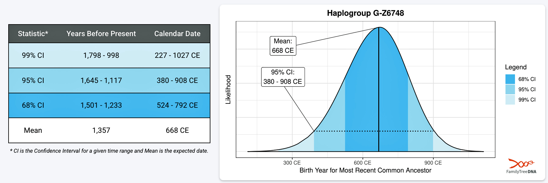
As indicated in previous parts of this story, the most recent common ancestor (MRCA) of haplogroup G-Z6748 may have been born around 668 CE. It is estimated that he had a 68 percent chance of being born between roughly 525 CE and 800 CE. [1] This 275 year time variance is not that big when attempting to pinpoint ancient DNA remains. [2] Illustration one depicts the archaeological time period of this roughly nine generation period or 275 year range of time.
Illustration One: Estimated Birth Date of tMRCA of G-Z6748, Archaeological Time, Periods, and Historical Events

During this 275 year period of time, the MRCA of G-Z6748 or preceding YDNA generations may have lived during the Early Medieval period B or the beginning of period C of the Early Medieval period. [3] These generations also lived at the end of the dark ages and during the ‘Great Migration’ when various social groups migrated in western Europe and specifically in the Netherlands area. It is also a period of time that witnessed shifting alliances and patterns of interaction and dominance between indigenous social groups from the post Roman era and emerging groups such as the Frisians, Franks and Saxons.
Between about 500 and 800 CE, the area of the later Netherlands lay in a fluctuating frontier zone where local post‑Roman populations, “new” Frisians inhabiting the North Sea coast, incoming Saxon groups in the northeast, and expanding Frankish power from the south interacted through shifting warfare, overlordship, and alliances. Multiple historical and archaeological studies explicitly frame this as a period of changing political configurations and changing social group relations rather than simple ‘ethnic’ group replacement. [4]

- The Ancestor of Haplogroup G-Z6748, the Terps, Transport Corridors and Landscape Archaeology – Part Eight January 14, 2026
- The Turbulent Roman Era – The Griff(is)(es)(ith) Y-DNA Phylogenetic Gap Associated with the Meuse and Rhine River Watershed – Part Seven November 30, 2025
- Looking at the Tail End of the Griff(is)(es)(ith) Y-DNA Phylogenetic Gap Associated with the Meuse and Rhine River Watershed – Part Six October 30, 2025
- Looking at the Griff(is)(es)(ith) Y-DNA Phylogenetic Gap Associated with the Meuse and Rhine River Watershed from the Bronze Age Onward – Part Five October 8, 2025
- Looking at the Griff(is)(es)(ith) Y-DNA Phylogenetic Gap Associated with the Meuse and Rhine River Watershed from the Bronze Age Onward – Part Four September 21, 2025
- Looking at the Griff(is)(es)(ith) Y-DNA Phylogenetic Gap Associated with the Meuse and Rhine River Watershed – Part Three August 29, 2025
- Looking at the Griff(is)(es)(ith) Y-DNA Phylogenetic Gap Associated with the Meuse and Rhine River Watershed – Part Two July 29, 2025
- Looking at the Griff(is)(es)(ith) Y-DNA Phylogenetic Gap Associated with the Meuse and Rhine River Watershed – Part One June 30, 2025
“In the 19th century, Dutch historians believed that the Franks, Frisians, and Saxons had populated and inhabited the Low Countries, but this theory fell out of favour in the 20th century. Due to the scarcity of written sources, knowledge of this period depends to a large degree on the interpretation of archaeological data. The traditional view of a clear-cut division between Frisians in the north and coast, Franks in the south and Saxons in the east has proven historically problematic. Archeological evidence suggests dramatically different models for different regions, with demographic continuity for some parts of the country and depopulation and possible replacement in other parts, notably the coastal areas of Frisia and Holland. ” [5]
Boom, Bust and Slow Recovery
As depicted in illustration one, based on various archaeological studies that have analyzed population fluctuation and density during this time period, the first millennium CE in the (present‑day) Netherlands shows a broadly shared “boom–bust–slow recovery” demographic pattern, with strong regional divergence in the depth and timing of the bust and the speed of recovery. Two major population highs have been documented and reconstructed: a middle Roman era peak (roughly AD 70–270) and a renewed rise in the early medieval period C (ca. AD 725–950). Illustration two provides a more detailed reconstruction of this pattern. in the Rhine-Meuse delta region. [6]
Between these, there is a pronounced demographic trough: a sharp decline from the later third century into the fifth century, after which population levels remain low for several centuries and never return to middle Roman values within the first millennium. [7] In the Rhine–Meuse delta, quantitative reconstructions indicate a rural population drop on the order of roughly 80 percent (ca. 78–85 percent) between the middle and late Roman periods.[8] ‘National‑ scale’ estimates suggest that a comparable late/post‑Roman decline affected much of what is now the present‑day Netherlands, though the magnitude of contraction varies between coastal, fluvial (landscapes associated with river systems), and inland sandy regions. [9]
Illustration Two: Reconstructed Palaeodemographic Trends for the Rhine-Meuse Delta During the First Millennium CE

This demographic trough coincides with the withdrawal of Roman military and administrative structures, larger general regional political instability, and increased flooding in parts of the fluvial zone. In the post-Roman era (the Early Middle Ages), the fluvial zone in the Netherlands was a highly dynamic, wet, and largely primitive landscape characterized by the environmental configuration of the Rhine-Meuse delta. It was an area of increased flooding, and significant shifting of river branches (avulsion). This period marked a transition from a Roman managed landscape to a more natural, water-dominated enivornmental area, particularly in the central Netherlands. [10]
After several centuries of low demographic levels, settlement numbers and inferred population start to rise again from roughly the later seventh to eighth century, with a clear demographic upswing in early medieval period C. By around 800 to 1000 CE, some regions (especially parts of the coastal and fluvial zone) are on a trajectory toward becoming among the most densely populated landscapes in northwest Europe, though still below the middle Roman peak in absolute terms for many areas. This recovery is tied to more stable political configurations, renewed agrarian exploitation of wetlands and floodplains, and large‑scale land reclamation and embankment processes that accelerates from the later first millennium into the high Middle Ages. [11]
Coastal and tidal marsh zones show strong late/post‑Roman contraction and, in some sectors, near‑abandonment, with relatively late reoccupation of specific areas on dwelling mounds and reclaimed grounds. The fluvial Rhine–Meuse area follows the classic boom–bust–slow recovery curve, with very high Roman densities, severe late Roman Era depopulation, and re‑growth from the eighth to ninth centuries onward as settlements shift to slightly higher levee positions under rising flood stress. Inland coversand and higher regions tend to show smaller population fluctuations. This area also witnesses the Roman‑era rise and post‑Roman decline, but with less dramatic contraction and sometimes earlier or smoother recovery relative to the low‑lying deltaic tracts of land. [12]
Various studies stress that demographic change was not a simple, uniform “collapse,” but a set of regionally differentiated trajectories produced by the interplay of political, economic, and environmental factors. [13] Through the use of high‑resolution, evidence‑ based demographic analysis (e.g. using ancient settlement inventories, large excavation datasets, and environmental proxies) these studies have provided a methodogical basis for explaining the spatial variation in cultural change and landscape transformation across the Roman–early medieval transition. [14]
The Migratory Path Among the Franks and the Frisians
As reflected in illustration one above, during and just prior to this 275 year period when the ancestor of haplgroup G-Z6748 lived, the Merovingian Dynasty became an emerging power. The Merovingians were a dynasty of Frankish kings who ruled much of what is now France, Belgium, western Germany, and parts of neighboring regions from the mid‑fifth century until they were replaced by the Carolingians in 751 CE. The northern border of the dynasty’s territory covered an area that included the migratory path of the ancestors of the MRCA of haplogroup G-Z6748 (see illustration two). [15]
Illustration Two: Map of the Rise and Expansion of the Merovingians, c. 639 CE

In addition to the Frankish Merovingian Dynasty, Frisian “power blocks”[16] , in what is now the northern Netherlands, crystallized as a coastal realm under kings or group leaders like Aldgisl and Radbod between roughly the mid‑seventh century and 734 CE. Their local dominance then fragmented under Frankish rule; and later re‑emerging as looser, more regional Frisian groups into the ninth and tenth centuries (see illustrations three through five). [17]
Illustrations Three, Four and Five: Various Stages of Magna Frisia
Illustration Three

Illustration Four

Illustration Five

Depending on where specific generations of the ‘immediate’ or preceding ancestors of the MRCA of G-Z6748 lived, they may likely have lived in areas controlled by groups identified as either Frisians or Franks. Based on the analysis of possible migratory corridors discussed in part eight of this story during this time period, illustration six depicts two possble migratory paths in the context of Frisian, Saxon and Frankish control.
In the context of the larger social and political influences, the genetic ancestors of the MRCA of G-Z6748 migrated through the Roman Limes area around the collapse of the Roman Empire, at a time and place that became increasingly controlled by the Frankish groups. These ancestors continued to move northward into areas inhabited by social groups known or identified as Frisians.
Illustration Six: Estimated Migratory Path of YDNA Ancestors and General Areas of Control by Frisians, Franks and Saxons Around 716 CE

A Period of Dynamic Interaction, Negotiated Power, and Evolving Identities among the Post‑Roman Communities
Archaeological evidence suggests dramatically different experiences for different regions, with demographic continuity for some parts of the area and depopulation and possible replacement in other parts, notably the coastal areas of Frisia. [18] The area that is currently the southern Netherlands experienced more continuity, with Frankish groups absorbing or mixing with remaining Romanized populations. Archaeological studies of late Roman and immediate post‑Roman settlement in the Low Countries stress continuity of local communities in parts of the river and loess zones, even as the coastal zone and nothern areas experienced major demographic change. This continuity in the southern area underlies the idea of “indigenous” post‑Roman groups (Franks) living in the river area interacting with incoming ‘re‑labelled’ Frisians and Saxons in the coastal and northern areas (see illustration seven). [19]
Illustration Seven: Approximate Positions of Indigenous Groups known from Roman Era Sources

During the third and fourth centuries, the population of Frisia steadily decreased, and by the fifth century it dropped dramatically. [20] The population decline of the Frisii was caused by flooding, disease and the fall of the Western Roman Empire. [21] The ancient indigenous groups—the Frisii, Batavians, and Cananefates who had lived under or alongside Roman rule—largely disappeared from the northern Netherlands. Archaeological surveys indicate that only small pockets of the original population stayed behind in areas like the Groningen coastal marshes, while coastal lands remained largely unpopulated for the next one or two centuries. [22]
Studies of the Anglo‑Saxon and Frisian migrations into the coastal Netherlands argue that new groups (Angles, Saxons, Franks) moved into lands formerly inhabited by the ancient Frisii, Cananefates and Batavians. Merovingian Frankish groups ‘retrospectivey’ labeled these mixed coastal populations “Frisians,” which itself points to a dynamic social reconfiguration of identities over the fifth through seventh centuries. [23]
Relationships between Frankish and Frisian areas in the Netherlands were highly porous in economic, social, and cultural terms, even while political and military conflicts periodically hardened boundaries between the groups. Archaeological and anthropological studies during this time period generally treat the Rhine–Meuse delta and coastal Netherlands as a long‑term contact zone rather than a firm frontier between two closed ethnic blocks. [24]
From an archaeological and anthropological standpoint, the Frankish–Frisian relationship in the Netherlands is best described as a semi‑porous frontier:
- Politically: there were real contests and shifting borders, especially around major river‑mouth centers; [25]
- Economically and socially: trade, mobility, mixed communities, and shared religious and legal frameworks created strong cross‑border connectivity; [26] and
- Ethnically and culturally: identities were fluid and situational, with overlapping Frankish and Frisian social spheres rather than sealed or self-contained cultural groups. [27]
Written sources and archaeology show alternating phases of Frankish expansion, Frisian autonomy, and shifting overlordship in the central river area (e.g. the Utrecht–Dorestad region) in the seventh–eighth centuries. [28] Studies of Dorestad and neighboring sites describe the Rhine delta as a frontier where Franks and Frisians “came to oppose each other,” yet this opposition coexisted with dense cross‑border interaction. The so‑called Frisian– Frankish wars underscore competition over key emerging ‘town settlements‘ like Utrecht and Dorestad in the river lowland area, but modern scholarship emphasizes that these conflicts did not create impermeable ethnic or social barriers. [29]
Studies on Merovingian and early Carolingian political geography emphasizes that Frisians could function both as rivals and as allies or clients of the Franks, depending on local rulers and phases of expansion, showing that power relations were contingent and negotiable rather than strictly binary. [30] Broader studies of cross Channel and North Sea politics in the sixth to seventh centuries (e.g. on Frankish–Britain relations) explicitly reject simple hegemonic models in favor of “balance of power” and “complex influence” frameworks to descibe the intergroup relationships. [31] The same authors of these studies apply similar concepts to North Sea coastal regions including Frisia, underlining that elite strategies involved selectively displaying Frankish connections, trading, and raiding in a fluid political environment. [32]
The Impact of the Great Migration During this Time Period
The term ‘Migration Period’ in Europe has been predominately used to refer to the ‘Migration Period’ (around 300-800 CE), when Germanic and other ‘tribes’ or groups reshaped Europe and were associated with the Western Roman Empire’s fall (see illustration seven). [33]
Illustration Seven: The Migration Period in Europe Fourth – Sixth Centuries CE

The Migration Period specifically refers to the important role played by the migration, invasion, and settlement of various social groups in western Europe, notably the Burgundians, Vandals, Goths, Alemanni, Alans, Huns, early Slavs, Pannonian Avars, Bulgars and Magyars within or into the territories of Europe as a whole and of the Western Roman Empire in particular. [34]
The Migration Period (circa 300–600 CE) fundamentally reshaped the Netherlands area as Germanic ‘tribes’ or aligned groups, including Franks, Saxons, and Frisians, moved into the crumbling Western Roman Empire’s northern territories. This triggered the abandonment of Roman-occupied southern areas of what is known as modern day Netherlands, leading to new cultural, linguistic, and political structures. [35]
All three of these groups were the result of early medieval ethnogenesis rather than direct continuation of Roman-period ‘tribes’ or indigenous groups. Archaeological studies also stress strong regional continuity from late Roman provincial and “native” communities, so these labels mask a heterogeneous population incorporating Batavian, Cananefatian, Chamavian and other pre-Roman / Roman-period indigenous groups (see side bar discussion on ethnogenesis).
New groups of Germanic peoples—primarily Saxons, along with Angles and Jutes—migrated into the northern regions. [36]. As mentioned above, the ‘ancient Frisii’ likely disappeared around 300 CE or the end of the third century due to coastal flooding and resettlement. [37] The newcomers who settled in the northern Netherlands adopted the name or were referred by outside groups by the name “Frisians,” though they were not descended from the ancient Frisii. These “new Frisians” became the ancestors of the medieval Frisian population.
Archaeological research suggests that the Migration Period brought an initial dramatic depopulation of specific areas, ecological and settlement reconfiguration, and later Frankish consolidation in what is now the Netherlands, rather than a simple “replacement” by incoming social groups.[38] The “Great Migration” in the area that is presently the Netherlands is partly visible as the absence of population: fewer sites, shorter occupation spans, and gaps in archaeological material culture rather than a clear mass-arrival new social groups. [39]

Ethnogenesis: Ethnicity, Tribes and Archaeology
Ethnogenesisis is the process by which a distinct ethnic group comes into being, emerges, or is formed, often arising from the blending, reformation, or interaction of existing groups, cultures, and populations. It involves the creation of a new, shared identity, frequently influenced by factors like migration, political changes, or social, economic, and historical experiences. [40]
Archaeologists have shifted from treating ethnogenesis as the simple “birth” of a fixed ethnic group to seeing it as an ongoing, contested process of identity making under specific historical and political conditions. Archaeologists in the late 20th century increasingly treated ethnicity as a relational process of boundary making rather than a bundle of traits. Ethnogenesis became a way to analyze how interaction, competition, and alliance in plural societies produced new ethnic boundaries, while highlighting internal heterogeneity and situational identities. [41]
Scholars highlight cycles of emergence, maintenance, transformation, and disappearance of ethnic identities (e.g., Hu’s concept of “ethnomorphosis”), pushing archaeologists to track identity work across multiple scales and articfacts (time, landscapes, and material practices).[42]
“Ethnic identities are always constructed in close association with political systems. It is politics that define ethnicity, not vice versa. Ethnic affiliation may be expressed at different scales of social organisation. At the highest level, there are macro-ethnic formations (Großstamme) such as Ionians and Achaians, or Gauls and Germans. At a local or regional level, smaller social groups may be discerned that coincide with localised political communities (e.g. poleis, civitates, or tribes). Despite frequent claims by ethnic groups to the contrary, all ethnic formations are intrinsically unstable and dynamic over time.” [43]
Read More on the Use of Terms “Ethnicity” and “Tribe” to Describe the Complexity and Fluidity of Groups Across the Late Prehistory and Early Historical Periods
Here is a breakdown of the movements that shaped this territorial map:
- Salian Franks (South/Central): Pushed by Saxons, the Salian Franks moved from the east over the Rhine into Roman territory in the fourth century. They settled in the Texandria region (modern-day Southwest Netherlands/North Brabant) as foederati (Roman allies) before establishing their base.
- Frisians (North/Coastal): Coastal areas, especially in the north, were occupied by the Frisians, who populated the coastal provinces. This area was known as Frisia Magna or Greater Frisia (illustration six).
- Saxons (East): Saxons pushed into the north eastern parts of the Netherlands with some Anglian/Jutish elements in the earliest coastal influx.
- De-population and Migration: The Roman border (Limes Germanicus), which ran along the Rhine, saw a significant reduction in population, with many settlements abandoned as the Roman army withdrew, leading to a largely rural, sparsely populated landscape in the center.
- The Power Shift: By the seventh and eighth centuries, a time when the MRCA of G-Z6748 lived, the region was contested between the Frisians in the north and the expanding Frankish Kingdom in the south, with major trading centers like Dorestad and Utrecht (Traiectum ad Rhenum) developing as key trading hubs.
The Migration Period’s impact in the lowlands and coastal areas is best understood as an extended period of demographic and environmental change, a reorganization of settlement systems, and a gradual emergence into a Frankish – Frisian and North Sea cultural network, rather than a series of discrete migratory events.
Overlapping, Shifting Power Blocs of Franks, Frisians, and Saxons
Between 400 and 800 CE, research scholarship sees Saxons, Frisians, and Franks in the Netherlands not as three sealed “tribes” or ‘ethnic groups’ but as overlapping, shifting power blocs whose relations ran through trade, warfare, and Frankish‑driven ethnogenesis.
If we consider the above mentioned 275 year time span that encompassed the time of birth for the most recent common ancestor of G-Z6748 or his ancestor, we can portray the the larger, general social context and general impact of the Migration Period on these roughly nine generations that lived in this time frame (see table one).
Table One: Political geography and ”Ethno’ Political Characterstics Over Time
Historians today tend to characterize the tri‑partite relationship in the Netherlands as:
- A Frankish hegemonic core pushing north;
- A Frisian maritime middle ground mediating trade and resisting, then accommodating Frankish power; and
- Saxon‑linked hinterlands interacting militarily and socially with both, later violently drawn into the Carolingian realm. [44]
Rather than three stable ethnic blocks, the literature treats them as fluid coalitions whose boundaries, political structures, and even names were repeatedly renegotiated through raids, alliances, Christianization, and the growing power of Frankish kings. The interaction is often framed as a long frontier struggle: campaigns by Frankish Merovingian and then Carolingian rulers to control northern tolls and convert Frisian and Saxon elites. [45] Frisian–Frankish wars in the seventh–eighth centuries end with Frisian defeat and incorporation; soon after, protracted Saxon wars extend similar Frankish domination eastward. [46] Nevertheless, studies emphasize continuity of local populations and laws (e.g. Lex Frisionum) under Frankish rule, suggesting integration through tribute, law‑codes, and missionary networks more than wholesale replacement. [47]
The Rhine–Meuse axis remains a political and fiscal frontier into the later seventh century, with successive shifts in control of key sites like Utrecht and Dorestad between Frankish and Frisian rulers before final Frankish consolidation. The Frisian–Frankish wars of the early eighth century, culminating in battles such as the Boarn (734 CE), bring most of the coastal Low Countries, including the northern parts of the watershed, into the Carolingian sphere. [48] From roughly the seventh century onward, a dense North Sea trading system linked Frisian, Frankish, and Saxon (in practice often Anglo‑Saxon and “Frisio‑Saxon”) communities into a single commercial zone. [49]
The Franks
The Franks first appear in the historical and archaeological record during the late Roman Empire, with evidence of interactions—often as raiders or federated allies (foederati) along the Roman frontier, especially in the lower Rhine region. [50] During the third to fifth centuries CE, Frankish groups increasingly settled within Roman territories, sometimes forcibly as a result of Roman policy (deportations or settlement of war captives), and sometimes through negotiation for land in exchange for military service. This led to a blending of Frankish and Gallo-Roman populations, as well as the transmission of Roman military, administrative, and material cultural practices to the newcomers. [51]
” ‘Franks’ is a Roman collective label for a series of smaller tribes in the areas east and north of the Lower Rhine who had long maintained relations with the Roman Empire. However, it wasn’t until the early 3rd century that they were given this name by the Roman authorities. The ethnicon ‘Franks’ was subject to change in the course of time, with the 3rd-century meaning differing considerably from that of the 5th century. . . . Frankish groups underwent a serious social transformation during the Late Roman period and that this was closely tied to increasing interaction – both friendly and hostile – with the Roman Empire. Viewed from this perspective, the Franks can be regarded as a ‘product’ of the complex dynamics in the Late Roman frontier.” [52]
The Franks rose to prominence in the centuries following the Roman era through processes of sociopolitical consolidation, adaptation to post-Roman contexts, and deep interaction with remaining Roman systems and populations. Archaeological and anthropological studies highlight their transformation from loosely organized tribal or indigenous groups into a dominant political force that shaped early medieval Western Europe.
“(T)he Frankish identity emerged at the first half of the 3rd century out of various earlier, smaller Germanic groups, including the Salii, Sicambri, Chamavi, Bructeri, Chatti, Chattuarii, Ampsivarii, Tencteri, Ubii, Batavi and the Tungri, who inhabited the lower and middle Rhine valley between the Zuyderzee and the river Lahn and extended eastwards as far as the Weser, but were the most densely settled around the IJssel and between the Lippe and the Sieg. The Frankish confederation probably began to coalesce in the 210s.“
“The Franks eventually were divided into two groups: the Ripuarian Franks (Latin: Ripuari), who were the Franks that lived along the middle-Rhine River during the Roman Era, and the Salians, who probably originated in the Salland in Overijssel, before pressure from the Saxons then forced them to move into the empire in the 4th century and became the Salian Franks.” [53]
The Salian and Ripuarian Franks emerge from the same broader Frankish confederation on the Rhine frontier, but they crystallize in different border zones and under different types of Roman interaction as reflected in table two and in illustration eight. [54]
Table Two: Summary Diferences Between Salian and Ripuarian Franks [55]
| Differences | Salian Frank | Ripuarian Frank |
|---|---|---|
| Origins | Earliest named in late Roman sources (Ammianus) as Franks “whom custom calls Salii,” living inside the Empire in Toxandria (southern Netherlands / Belgium between Meuse and Scheldt). They appear as a coastal and river‑delta frontier population, initially pirates/raiders, then foederati settled by Roman permission in the 4th century. [55a] | Their ancestors are ‘right‑bank’ Rhine peoples of the middle Rhine zone (Bructeri, Chamavi, Tencteri, Sicambri, Chattuarii, etc.) who gradually coalesce into a Frankish identity along the Cologne–Rhineland frontier. |
| Their pre‑Toxandrian homeland is obscure; one late source (Zosimus) says they had previously lived outside the Empire and were pushed into Batavia by Saxons, but modern scholarship treats them more as a new confederate label for groups already along the lower Rhine than as a single ancient “tribe.” [55b] | The name Ripuarii/Ribuarii is not definitively attested until the 7th–8th centuries, when it describes the Frankish population around Cologne and the lower/middle Rhineland; it is tied to a legal code (Lex Ribuaria) and a Merovingian regional category rather than to a clearly attested pre‑Merovingian “tribe.” | |
| Evidence & Timing | Pre‑Merovingian documentation is relatively good: Roman historians mention Salii explicitly in the 4th century, in a context of imperial settlement and frontier defense; by the 5th century they form the backbone of the lower‑Rhine Frankish polity of Chlodio and then the Merovingians. | Pre‑Merovingian evidence is indirect: Frankish groups are noted on the middle Rhine, but the specific label “Ripuarian” only surfaces clearly in Merovingian‑age legal and narrative sources; some scholars connect Jordanes’ Riparii at the Catalaunian Fields with them, but that identification is debated. |
| Frontier setting and Roman relationship | Lower Rhine / North Sea Delta: Strongly shaped by coastal defense politics, piracy, and Roman resettlement of Franks as laeti and foederati in depopulated frontier lands like Toxandria. Salian ethnogenesis is closely entangled with Roman military and agrarian policy on the lower Rhine limes border. | Middle Rhine / Cologne: Shaped by long‑term contact between Roman Cologne and right‑bank Germanic groups, with a mix of raiding, recruitment, and gradual Frankish penetration onto the left bank, culminating in control of Cologne in the 5th century. Their emergence as a named group reflects Merovingian re‑organization of this older Rhineland frontier population. |
| Later legal–regional codification | Lex Salica becomes the law code applied in much of northern Gaul between Loire and Silva Carbonaria, associated with the ruling Merovingian line of (ultimately) Salian background. | Lex Ribuaria (c. 7th century) governs the Rhineland around Cologne and seems to build on, or parallel, the legal traditions also reflected in Lex Salica, but framed for a distinct Austrasian/Rhenish jurisdiction. |
Illustration Eight: Frankish Expansion Between the Fourth and Ninth Centuries CE

Archaeologists Royens and Heeren provide a regional synthesis of archaeological and historical evidence from the Lower Rhine valley to illuminate how Roman and Frankish societies interacted and transformed during Late Antiquity. Their contention is the Franks are a Late Roman Era product. The Franks were not a long-standing ethnic group but rather a political-military formation emerging through Roman frontier interactions. Their rise was deeply entangled with Roman systems of payment, alliance, and warfare. By the fifth century, Frankish warlords had consolidated local power in former Roman territories, adopting Roman offices, titles, and material culture to legitimize their authority. [56]
These populations mixed with local survivors, forming a “hybrid Romano-Frankish frontier culture” rather than replacing the old one entirely. Archaeological evidence, such as distinct house types, weapon forms (like the francisca), and dress accessories, indicates the arrival of new population groups—likely from north of the Rhine (Elbe-Weser and Drenthe/Veluwe regions). The authors analyze a remarkable surge of gold hoard deposits found in the Lower Rhine area in the late fourth to fifth centuries. These hoard deposits are interpreted as payments to Frankish foederati, i.e., allied warbands employed by the Empire. Estimates suggest several thousand kilograms of gold circulated, showing substantial imperial investment in frontier diplomacy and defense. [57]
“There is general agreement that gold circulation in Late Roman frontier regions was closely bound up with the military sphere as payment to soldiers and to leaders of federate war bands. The Late Roman gold influx into the Lower Rhine region reflects payments by the Roman authorities or usurpers to Frankish allies (foederati) in exchange for military support. “ [58]
“The temporal patterning of the gold influx also prompts some interesting observations. Four phases can be distinguished, based on the dating of the hoard finds (illustration nine) . We see a modest beginning in the third quarter of the 4th century, followed by a clear peak in the early 5th century. The number then falls again in the second quarter of the 5th century, before disappearing after a final hoard in c. 460 AD. Another interesting development is the spatial distribution of hoards over time. The earliest hoards are concentrated in the area east of the Rhine. In the early 5th century they went on to cover the area both east and west of the Lower Rhine.” [59]
Illustration Nine: Distribution of Late Roman Gold Hoards

Royens and Heeren reject simple narratives of “Roman decline.” Instead, they emphasize continuity through transformation—the shift from Roman provincial society to early Frankish polities resulted from adaptive processes and mixed communities along the frontier. [60]
Archaeological evidence suggests that Frankish society underwent marked militarization and increasing social hierarchy during the Late Roman period. This process was driven by both conflict and cooperation with Rome. Access to Roman arms, fortifications, and wealth enhanced Frankish capacity for warfare and power brokerage, while the decline of centralized Roman authority created a vacuum for ambitious leaders to exploit. By the late fifth century, the Franks—especially under leaders such as Clovis—united previously disparate tribal groups to form the Merovingian dynasty, consolidating power in northern Gaul and moving towards the creation of a kingdom. [61]
Once established in former Roman Gaul, the Franks showed notable adaptability. They integrated aspects of Roman culture, language, law, and administrative practice, and adopted Christianity, which aided legitimization among local elites and the Church. Archaeological studies of burial practices, settlement patterns, and material culture reflect both continuity and innovation—a pragmatic retention of certain Roman traditions (e.g. urban lay-out, Christian sites) alongside distinctively Frankish elements (weapon graves, personal adornment styles). [62]
Early Medieval Frisians and Saxons
Along the terp and salt-marsh zone of the northern Netherlands, post‑Roman reoccupation and expansion during the fifth through seventh centuries is archaeologically associated with the emergence of a new Frisian kingdom or confederation. Linguistic and archaeological studies emphasize that these “new Frisians” drew on Anglo‑Saxon–like migrant groups and surviving coastal populations. They were not a simple continuation of the Roman-period Frisii tribe. [63]
These “new Frisians” descended largely from Saxon-, Angle- and Jute‑rich migrant streams mixed with remaining coastal populations, rather than directly from the Roman‑period Frisii. [64] As part of the the early Migration‑Period inflow into the northern Low Countries; many of the Angles and Jutes moved on to Britain as “Anglo‑Saxons”, but some remained within the coastal zone that became Frisia.
On the basis of settlement archaeology, archaeologist Jos Bazelmans argues that there was a marked break in habitation in the terp and marsh areas of present‑day Friesland between the later third and fifth centuries. This hiatus suggests that the Roman‑period Frisii of the northern Dutch coastal zone did not form a continuous, sedentary population that simply “became” the early‑medieval Frisians. The re‑occupation of the region in the fifth–sixth centuries is interpreted as involving new or restructured population groups, rather than the uninterrupted survival of a Roman‑era ethnic community. The mediaval Frisians were the result of a later, politically driven reuse of an old ethnonym by the Frankish elite, superimposed on a population that had undergone substantial demographic and cultural discontinuity. [65]
Bazelmans starts from two puzzles: the disappearance of the ethnonym ‘Frisii ‘from late Roman written sources after the third century, and its reappearance as Frisii/Frisones and Frisia in Merovingian and Carolingian texts from the sixth–seventh centuries onward. Bazelmans combines (1) archaeological settlement history in present‑day Friesland, (2) the textual tradition on the Frisiiand early‑medieval Frisians, and (3) comparative work on how imperial centers create and recycle ethnonyms on their frontiers.
Because the ethnonym disappears from the written record for roughly three centuries and then reappears attached to a reorganized coastal frontier, Bazelmans concludes that the name Frisia/Frisii was reintroduced from the outside, rather than preserved locally as an unbroken self‑designation. He suggests that Merovingian Frankish elites, drawing on the Roman ethnographic tradition, revived the old name for administrative and ideological purposes when integrating the coastal zone into a Frankish frontier system in the seventh century.
In this reading, the ethnonym “Frisians” is a product of imperial categorization. The Franks used the prestigious Roman repertoire of peoples at the North Sea coast to label and order frontier populations, thereby projecting Roman antiquity onto a new political geography. Dusting off and reusing the name Frisia could also have served practical purposes, for example in asserting claims over former Roman state land or legitimising Frankish authority in a region framed as an old Roman periphery.
Bazelmans’ main theoretical conclusion is that continuity of an ethnic name in texts does not necessarily imply continuity of population, culture, or self‑identification on the ground. The Frisian case shows how an old ethnonym can be revived after a demographic and textual gap, filled with new content, and then become internalized by later inhabitants to the point that it underpins strong regional and national narratives. For early‑medieval ethnicity, he urges treating ethnonyms as historically contingent labels embedded in power relations and Roman-Frankish discursive traditions, rather than as straightforward reflections of long‑lived “peoples.”
There is no wholesale refutation of Bazelmans arguments, but several scholars nuance or push back against specific parts of his model: the strength of the demographic “break,” the degree of Frankish top‑down control over the ethnonym, and whether “Frisian” is best read as primarily political rather than an ethnic entity. Some work on Frisian and Saxon “mirror histories” accepts the textual gap Bazelmans highlights but is more cautious about turning this into a hard population rupture, stressing that limited sources make any sharp discontinuity model fragile. Instead of a simple break and replacement, these authors emphasize overlapping coastal populations, flexible identities, and the possibility that at least some late Roman groups persisted under changing labels. [66]
IJssennagger‐Van der Pluijm explicitly cites Bazelmans’ view—that “Frisian” was re‑established by the Franks as a political term—but suggests an alternative reading in which Frisia is used “primarily as a geographical term” for a coastal zone, with Frisii/Frisones referring broadly to its inhabitants. This shifts the emphasis away from a purely invented, top‑down ethnic category toward a more open, regional label that could carry ethnic, political and geographical meanings simultaneously. [67]
Archaeological papers that were published in the same ‘Ethnic Constructs in Antiquity’ volume that includes Bazelman’s paper and later debates over ethnonyms stress that externally imposed labels are regularly appropriated and reworked “from below,” and some scholars think Bazelmans underplays this local agency in the early phases. On this view, even if the Frankish elite reintroduced the name from Roman tradition, coastal communities quickly began to fill “Frisian” with their own content, so the label cannot be treated as merely imperial shorthand or a passive political tag. [68]
Some historians and linguists are uneasy with treating “Frisian” mainly as a political category, arguing that law, language and mythic history in later Old Frisian texts reveal a strong sense of gens, or group identity, shaped by shared customs and a sacred past. From this angle, Bazelmans’ stress on power and discontinuity risks underestimating the emergence of a genuine ethnic self‑understanding by the High Middle Ages, even if the name’s reactivation was conditioned by Merovingian and Carolingian politics. [69]
The End of the Phlogenetic Gap: Profound Changes Along the Migratory Path
This multipart story focused on examining a range of methdologiclal, macro social-cultural and enviromental influences that may help explain or put into context the lack of identified subclades (YDNA genetic ancestors) in the migratory path of the Griffis genetic paternal line. The period of time for this phylogenetic gap is roughly between 3000 BC and 650 CE.
Based on historical and archaeological studies, migrating generations associated with the tail end of this gap, between 525 and 800 CE, from the Rhine-Meuse delta to the northern coastal areas of the Netherlands (Frisia), would have experienced a profound transformation in lifestyle, moving from a formerly Romanized, partly abandoned riverine landscape to a dynamic, maritime-oriented, and largely independent society.
In terms of the environment, the Rhine–Meuse zone offered relatively stable riverine landscapes with levees, older settlements, and a mix of arable fields, pastures, and woodland. Generations heading north would face a different enviroment. The northern coast (Frisia and adjacent marshlands) was a low, flat salt‑marsh environment facing the North Sea, with tidal creeks, peat, and frequent flooding, so settlements clustered on artificial dwelling mounds (terpen) or natural ridges. [70]
In terms of settlements and housing conditions, the late Roman and post‑Roman communities in the river area often occupied slightly higher sand ridges and former Roman‑era sites, with dispersed farmsteads that gradually coalesced into villages. In the north, migrants would adapt to terp‑based settlement: compact farm clusters on raised mounds, surrounded by open marsh pasture and drainage channels, with periodic rebuilding and heightening after floods. [71]
The nature of subsistence and the local economies were different given the projected migratory path. The Rhine–Meuse delta supported mixed farming (e.g. grain, cattle, pigs) and benefited from proximity to former Roman markets and transport along major rivers. On the northern coast, life was more strongly oriented to cattle raising on rich salt‑marsh pastures, peat and salt exploitation, and coastal/riverine trade. Harvests were higher than on sandy inland soils but depended on successful drainage and protection from the sea. From the seventh–eighth centuries, the Frisian coastal zone participated in a North Sea trade network linking Britain, Francia, and Scandinavia, so the migrants associated with the YDNA lineage may have been were drawn into longer‑distance commerce in wool, cattle, and crafted goods.[72]
Riverine life involved flood risk, but it was more localized and structured by known river channels and levees. On the coast, people faced storm surges, occasional catastrophic inundations, and brackish water, so flood anxiety and ritual or communal responses to the sea were central to experience. [73] Standing water, peat, and marshes increased exposure to fevers (often interpreted as malaria‑like “agues”) and nutritional stress when storms damaged pasture or salinized fields. [74]
In the fifth and sixth centuries the Rhine–Meuse region was a frontier zone influenced by the fading Roman limes and the expanding Frankish kingdoms, with emerging local elites tied to Frankish power structures. The northern coastal belt from the Scheldt to the Weser was identified in early medieval sources as “Frisia,” a patchwork of Frisian petty kingdoms and communities, only gradually drawn under Frankish control in the seventh–eighth centuries. [75]
People leaving the Rhine–Meuse zone would move from a landscape with lingering Roman material culture and early Frankish Christian influence toward a Frisian cultural sphere that remained predominantly pagan until missionary efforts intensified in the seveth–eighth centuries. Over generations, migrants could shift language and identity from more Frankish‑oriented dialects toward Frisian (part of the Anglo‑Frisian group), participating in shared styles of dress, burial, and craftsmanship that linked communities around the North Sea. [76] In the early Middle Ages, Christian influence spread earliest and most densely in the south of what is now the Netherlands, somewhat later and more unevenly in the central river area, and last and most sporadically in the northern coastal/Frisian zone. [77]
. . . And What about the Phylogenetic YDNA Gap?
A Y‑DNA phylogeny showing long internal branches with few subclades, similar to the lack of known identified haplogroups over a long perod of time, is most consistent with a small, relatively isolated male lineage that expanded slowly and experienced limited splitting. This phylogenetic pattern can conceivably fit a scenario of repeated but low‑level (localized migration and local patrilocality on the northern Dutch coast between 500 and 800 CE. [78]
Long branches with minimal subclade formation usually imply either: (1) a long period with low effective male population size (drift, bottleneck, founder effect), or (2) a long period with low mutation “visibility” (few lineages sampled, or technical/mutation‑rate issues), or both. [79] In demographic terms this often reflects a founding male, or very few males, whose patriline persists for many generations with little diversification, either because few male lines exist, many side‑branches go extinct, or later expansions are recent and not yet phylogenetically resolved. [80]
If a small group of related males moved from the Rhine–Meuse zone into one or more terp communities and then remained largely endogamous and patrilocal, their Y‑line could show a long, “thin” branch: one main stem, few long‑lived offshoots. [81] Archaeology suggests reoccupation and growth of some northern terps after an earlier decline, consistent with founder events at the ‘village level’. A few successful founding patrilines could dominate local Y‑DNA distribution, producing deep but sparsely subdivided branches in subsequent subclades or branches of the genetic tree. [82]
Imagine one or two brothers from the Rhine–Meuse area settle on a terp around 600 CE. Of perhaps there was a succession of a few generations that slowly moved north-westward to the northern coast during this time period. Over a couple of centuries their male descendants remain in the same marsh community or they migrate to the English Isle in the context of the growing maritime trade, while collateral lines frequently die out or are replaced, leaving a single, long main Y‑line with few enduring splits.
Migration here is likely repetitive and small‑scale (family‑level, chain migration) rather than massive, so each episode may add only a few males; many incoming lines will be lost by drift, disease, or social disadvantage, leaving only one or two that survive into the future. [83] Technically, long branches with few observed splits can also reflect undersampling of the lineage, uneven marker discovery, or branch‑length artefacts in current Y references, so some “missing” subclades might be methodological rather than historical. [84]
Perhaps this last paragraph succinctly captures why there is this 2,850 year gap or absence of documented YDNA haplogroups in the genetic YDNA paternal line leading up to the Most Recetn Common ancestor of haplogroup G-Z6748: small scale family level chain migration and methodological artifact.
Sources:
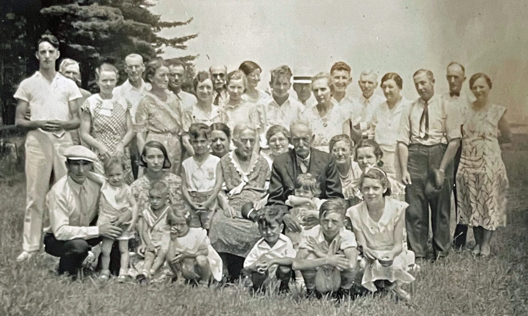
Feature Image: The left hand image is the scientific details for the estimated birth date for the most recent common ancestor associated with haplogroup G-Z6748. The right hand map is a map of Magna Frisia in Latin from Wikimedia Commons, https://commons.wikimedia.org/wiki/File:Frisia_716-la.svg. Magna Frisia (Greater Frisia) refers to an independent Frisian kingdom that existed in the coastal regions of the Netherlands and Germany from approximately 600–734 AD, during the Early Middle Ages. At its peak, it spanned from the Zwin near Bruges in Belgium to the Weser River in Germany. Perhaps the Most Recent Common Ancestor of G-Z6748 was born in Greater Frisia.
[1] Scientific Details for G-Z6748
[2] Estimating the precise birth year of ancient human remains using only haplogroups is highly difficult and generally not possible with high precision, often resulting in uncertainties of hundreds or thousands of years. While haplogroups can provide a general, deep ancestral timeframe (e.g., thousands of years ago), determining when a specific individual lived requires combining genetic data with other methods like radiocarbon dating.
Molecular Clock Variability: Haplogroup ages are estimated by counting SNP mutations (Single Nucleotide Polymorphisms – the common variations in the DNA sequence) and assuming a constant rate. However, mutation rates can vary, leading to different estimations depending on the model.
Evolutionary Time vs. Genealogical Time: A haplogroup’s “formation” date (when the mutation first appeared) is not the same as the birth year of a specific person in that lineage.
Factors Affecting Precision:
Haplogroup Resolution: High-resolution tests (e.g., Big Y) can narrow down a lineage to a few hundred years, but many standard tests only identify high-level, ancient branches (e.g., J-CTS5368, which is 19,000 years old).
Age of the Sample: The older the remains, the less accurate the specific birth year, while more recent remains (e.g., under 1,000 years) are easier to place if they belong to a well-defined, young branch.
Contamination and Quality: Ancient DNA often suffers from degradation or contamination, making it hard to identify specific, recent downstream SNPs, which limits accuracy.
For genealogical purposes (e.g. the (last ~500 years), haplogroups are difficult to use for precise birth years on their own. For archaeology, they are useful for identifying ancestral, migration-based, and broadly defined, ancient timeframes.
McDonald I. Improved Models of Coalescence Ages of Y-DNA Haplogroups. Genes (Basel). 2021 Jun 4;12(6):862. doi: 10.3390/genes12060862. PMID: 34200049; PMCID: PMC8228294, https://pmc.ncbi.nlm.nih.gov/articles/PMC8228294/
[3] The division of the Early Medieval era (roughly 500–1000 AD) into different “a,b,c, & d” periods or sub-phases (such as Early, Middle, and Late Saxon, or regional archaeological phases) exists because historians and archaeologists need to break down 500 years of complex, non-linear change into manageable, analytical units. Because historical, social, and cultural changes did not happen simultaneously across all of Europe, these subdivisions are necessary to reflect specific, localized developments.
The lettered phases (A–D) in Pierik’s article are not necessaily an universal scheme for the Early Middle Ages. It belongs to specific regional or thematic chronology and each such system defines A–D differently by artefact style, burial practice, and absolute dates.
The four periods A–D are defined as successive blocks within the first millennium AD, distinguished mainly by dominant landscape processes, regional geomorphological configurations, and the intensity and form of human land use across the Dutch coastal plain, river area, and Pleistocene sands. Pierik’s four periods are defined by absolute calendar dates and shifts in population trends and human impact on geomorphology, following an established Early Medieval A–D scheme used in related archaeological work.
See:
Pierik HJ. Landscape changes and human–landscape interaction during the first millennium AD in the Netherlands. Netherlands Journal of Geosciences, Volume 100, e11. https://doi.org/10.1017/njg.2021.8
Pierk, H.J. and Rowin J. van Lanen, Roman and early-medieval habitation patterns in a delta landscape: The link between settlement elevation and landscape dynamics, Quaternary International xxx (2017) 1e14, https://www.academia.edu/34741833/Pierik_and_Van_Lanen_2017_Roman_and_early_medieval_habitation_patterns_in_a_delta_landscape_The_link_between_settlement_elevation_and_landscape_dynamics
[4] History of the Netherlands, Wikipedia, This page was last edited on 21 January 2026, https://en.wikipedia.org/wiki/History_of_the_Netherlands
Netherlands in the Early Middle Ages, Wikipedia, This page was last edited on 2 December 2025, https://en.wikipedia.org/wiki/Netherlands_in_the_Early_Middle_Ages
Low Countries, Wikipedia, This page was last edited on 29 November 2025, https://en.wikipedia.org/wiki/Low_Countries
Kooijmans, Leendert P. Louwe, Kieft, C. van de, Blockmans, Wim. “history of the Low Countries”. Encyclopedia Britannica, 29 Jul. 2022, https://www.britannica.com/topic/history-of-the-Low-Countries-prehistoric-times-to-1579-2157575
Bavuso, I. (2021) Balance of power across the Channel: reassessing Frankish hegemony in southern England (sixth–early seventh century). Early Medieval Europe, 29: 283–304. https://doi.org/10.1111/emed.12481
Wallace-Hadrill, John Michael, Heather, Peter John, Bayley, Charles Calvert, Berentsen, William H., Turner, Henry Ashby, Sheehan, James J., Hamerow, Theodore S., Duggan, Lawrence G., Elkins, Thomas Henry, Geary, Patrick J., Leyser, K.J., Strauss, Gerald, Kirby, George Hall, Schleunes, Karl A., Barkin, Kenneth. “Germany”. Encyclopedia Britannica, 27 Jan. 2026, https://www.britannica.com/place/Germany .
Fierman, Roberrt, Mirror Histories: Frisians and Saxons from the First to the Nineth Centruty AD, in Edited by John Hines, Nelleke IJssennagger-van der Pluijm (eds), Frisians of the Early Middle Ages. Boydell & Brewer; 2021. 223-248., https://research-portal.uu.nl/ws/portalfiles/portal/232053797/mirror-histories-frisians-and-saxons-from-the-first-to-the-ninth-century-ad.pdf
Beyen, Marnix, A Tribal Trinity: The Rise and Fall of the Franks, the Frisians and the Saxons in the Historical Consciousness of the Netherlands since 1850 , European History Quarterly, 30(4), 2000, 493-532. https://doi.org/10.1177/026569140003000402 (Original work published 2000) https://library.fes.de/libalt/journals/swetsfulltext/8798011.pdf
Netherlands in the Early Middle Ages, Wikipedia, This page was last edited on 2 December 2025, https://en.wikipedia.org/wiki/Netherlands_in_the_Early_Middle_Ages
Reimersa, Franz, Is Magna Frisia Fact or Fiction?, Frisia Coast Trail Blog, https://www.frisiacoasttrail.com/post/2018/09/01/is-magna-frisia-fact-or-fiction
Lyra Mapping, The history of the Netherlands, every year, 2017, YouTube, https://www.youtube.com/watch?v=TUWqYaEm4h8

Schuffelen, Marco, Historical Maps of The Netherlands (“Holland”), Holland Timeline, (Maps of Netherlands 300 AD and 100 AD), 2009, https://www.heardutchhere.net/NLtimeline.html
Ealdlar, Anglo-Frisian Origins: Shared Heritage Across the North Sea, 22 May 2025, Ealdlar, https://ealdlar.com/history/anglo-frisian-origins
[6] History of the Netherlands, Wikipedia, This page was last edited on 21 January 2026, https://en.wikipedia.org/wiki/History_of_the_Netherlands
[7] van Lanen RJ, de Kleijn MTM, Gouw-Bouman MTIJ, Pierik HJ. Exploring Roman and early-medieval habitation of the Rhine–Meuse delta: modelling large-scale demographic changes and corresponding land-use impact. Netherlands Journal of Geosciences. 2018;97(1-2):45-68. doi:10.1017/njg.2018.3, https://www.cambridge.org/core/journals/netherlands-journal-of-geosciences/article/exploring-roman-and-earlymedieval-habitation-of-the-rhinemeuse-delta-modelling-largescale-demographic-changes-and-corresponding-landuse-impact/40F68343AEEC8FF41124C5F098069863
van Lanen, Rowin J., and Bert Groenewoudt, Counting heads: Post-Roman population decline in the Rhine-Meuse delta (the Netherlands) and the need for more evidence-based reconstructions, in Niall Brady and Claudia Theune, eds, Across Medieval Europe: Old Paradigmsand New Vistas, Ruralia XII, Lieden: Sidestone Press, 2019, 113- 134, https://www.academia.edu/40523376/Counting_heads_Post_Roman_population_decline_in_the_Rhine_Meuse_delta_the_Netherlands_and_the_need_for_more_evidence_based_reconstructions
[8] van Lanen RJ, de Kleijn MTM, Gouw-Bouman MTIJ, Pierik HJ. Exploring Roman and early-medieval habitation of the Rhine–Meuse delta: modelling large-scale demographic changes and corresponding land-use impact. Netherlands Journal of Geosciences. 2018;97(1-2):45-68. doi:10.1017/njg.2018.3, https://www.cambridge.org/core/journals/netherlands-journal-of-geosciences/article/exploring-roman-and-earlymedieval-habitation-of-the-rhinemeuse-delta-modelling-largescale-demographic-changes-and-corresponding-landuse-impact/40F68343AEEC8FF41124C5F098069863
van Lanen, Rowin J., and Bert Groenewoudt, Counting heads: Post-Roman population decline in the Rhine-Meuse delta (the Netherlands) and the need for more evidence-based reconstructions, in Niall Brady and Claudia Theune, eds, Across Medieval Europe: Old Paradigmsand New Vistas, Ruralia XII, Lieden: Sidestone Press, 2019, 113- 134, https://www.academia.edu/40523376/Counting_heads_Post_Roman_population_decline_in_the_Rhine_Meuse_delta_the_Netherlands_and_the_need_for_more_evidence_based_reconstructions
Groenewoudt, Bert and Rowin J. van Lanen, Diverging decline : reconstructing and validating (post-)Roman population trends (AD 0-1000) in the Rhine-Meuse delta (the Netherlands), PCA, European journal of postclassical archaeologies, vol. 8 (2018), p 189-218, https://www.researchgate.net/publication/327867127_Diverging_decline_Reconstructing_and_validating_post-Roman_population_trends_AD_0-1000_in_the_Rhine-Meuse_delta_the_Netherlands
[9] van Lanen RJ, de Kleijn MTM, Gouw-Bouman MTIJ, Pierik HJ. Exploring Roman and early-medieval habitation of the Rhine–Meuse delta: modelling large-scale demographic changes and corresponding land-use impact. Netherlands Journal of Geosciences. 2018;97(1-2):45-68. doi:10.1017/njg.2018.3, https://www.cambridge.org/core/journals/netherlands-journal-of-geosciences/article/exploring-roman-and-earlymedieval-habitation-of-the-rhinemeuse-delta-modelling-largescale-demographic-changes-and-corresponding-landuse-impact/40F68343AEEC8FF41124C5F098069863
van Lanen, Rowin J., and Bert Groenewoudt, Counting heads: Post-Roman population decline in the Rhine-Meuse delta (the Netherlands) and the need for more evidence-based reconstructions, in Niall Brady and Claudia Theune, eds, Across Medieval Europe: Old Paradigmsand New Vistas, Ruralia XII, Lieden: Sidestone Press, 2019, 113- 134, https://www.academia.edu/40523376/Counting_heads_Post_Roman_population_decline_in_the_Rhine_Meuse_delta_the_Netherlands_and_the_need_for_more_evidence_based_reconstructions
[10] Groenewoudt, Bert and Rowin J. van Lanen, Post-Roman population dynamics in the Rhine- Meuse delta (the Netherlands). RURALIA XII Conference, 11th-17th September, Kilkenny (Ireland), https://www.academia.edu/34604939/Post_Roman_population_dynamics_in_the_Rhine_Meuse_delta_the_Netherlands_RURALIA_XII_Conference_11th_17th_September_Kilkenny_Ireland_
Groenewoudt, Bert and Rowin J. van Lanen, Diverging decline. Reconstructing and validating (post-) Roman population trends (AD 0-1000) in the Rhine-Meuse delta (the Netherlands), PCA 8 (2018) ISSN: 2039-7895 (pp. 189-218), https://www.postclassical.it/PCA_Vol.8_files/PCA8_Groenewoudt-VanLanen.pdf
[11] Pierik, Harm Jan, Landscape changes and human–landscape interaction during the first millennium AD in the Netherlands, Netherlands Journal of Geosciences, Volume 100, e11. https://doi.org/10.1017/njg.2021.8
[12] Pierik, Harm Jan, Landscape changes and human–landscape interaction during the first millennium AD in the Netherlands, Netherlands Journal of Geosciences, Volume 100, e11. https://doi.org/10.1017/njg.2021.8
[13] Pierik, Harm Jan, Landscape changes and human–landscape interaction during the first millennium AD in the Netherlands, Netherlands Journal of Geosciences, Volume 100, e11. https://doi.org/10.1017/njg.2021.8
Groenewoudt, Bert and Rowin J. van Lanen, Diverging decline. Reconstructing and validating (post-) Roman population trends (AD 0-1000) in the Rhine-Meuse delta (the Netherlands), PCA 8 (2018) ISSN: 2039-7895 (pp. 189-218), https://www.postclassical.it/PCA_Vol.8_files/PCA8_Groenewoudt-VanLanen.pdf
[14] Groenewoudt, Bert and Rowin J. van Lanen, Diverging decline : reconstructing and validating (post-)Roman population trends (AD 0-1000) in the Rhine-Meuse delta (the Netherlands), PCA, European journal of postclassical archaeologies, vol. 8 (2018), p 189-218, https://www.researchgate.net/publication/327867127_Diverging_decline_Reconstructing_and_validating_post-Roman_population_trends_AD_0-1000_in_the_Rhine-Meuse_delta_the_Netherlands
Groenewoudt, Bert and Rowin J. van Lanen, Post-Roman population dynamics in the Rhine- Meuse delta (the Netherlands). RURALIA XII Conference, 11th-17th September, Kilkenny (Ireland), https://www.academia.edu/34604939/Post_Roman_population_dynamics_in_the_Rhine_Meuse_delta_the_Netherlands_RURALIA_XII_Conference_11th_17th_September_Kilkenny_Ireland_
van Lanen RJ, de Kleijn MTM, Gouw-Bouman MTIJ, Pierik HJ. Exploring Roman and early-medieval habitation of the Rhine–Meuse delta: modelling large-scale demographic changes and corresponding land-use impact. Netherlands Journal of Geosciences. 2018;97(1-2):45-68. doi:10.1017/njg.2018.3, https://www.cambridge.org/core/journals/netherlands-journal-of-geosciences/article/exploring-roman-and-earlymedieval-habitation-of-the-rhinemeuse-delta-modelling-largescale-demographic-changes-and-corresponding-landuse-impact/40F68343AEEC8FF41124C5F098069863
[15] van Lanen RJ. Revealing the past through modelling? Reflections on connectivity, habitation and persistence in the Dutch Delta during the 1st millennium AD. Netherlands Journal of Geosciences. 2020;99:e14. doi:10.1017/njg.2020.12, https://www.cambridge.org/core/journals/netherlands-journal-of-geosciences/article/revealing-the-past-through-modelling-reflections-on-connectivity-habitation-and-persistence-in-the-dutch-delta-during-the-1st-millennium-ad/717D79192E8EDD6B90D58B060117EB1B
Groenewoudt, Bert and Rowin J. van Lanen, Post-Roman population dynamics in the Rhine- Meuse delta (the Netherlands). RURALIA XII Conference, 11th-17th September, Kilkenny (Ireland), https://www.academia.edu/34604939/Post_Roman_population_dynamics_in_the_Rhine_Meuse_delta_the_Netherlands_RURALIA_XII_Conference_11th_17th_September_Kilkenny_Ireland_
Groenewoudt, Bert and Rowin J. van Lanen, Diverging decline : reconstructing and validating (post-)Roman population trends (AD 0-1000) in the Rhine-Meuse delta (the Netherlands), PCA, European journal of postclassical archaeologies, vol. 8 (2018), p 189-218, https://www.researchgate.net/publication/327867127_Diverging_decline_Reconstructing_and_validating_post-Roman_population_trends_AD_0-1000_in_the_Rhine-Meuse_delta_the_Netherlands
Pierik, Harm Jan, Landscape changes and human–landscape interaction during the first millennium AD in the Netherlands, Netherlands Journal of Geosciences, Volume 100, e11. https://doi.org/10.1017/njg.2021.8
van Lanen RJ, de Kleijn MTM, Gouw-Bouman MTIJ, Pierik HJ. Exploring Roman and early-medieval habitation of the Rhine–Meuse delta: modelling large-scale demographic changes and corresponding land-use impact. Netherlands Journal of Geosciences. 2018;97(1-2):45-68. doi:10.1017/njg.2018.3, https://www.cambridge.org/core/journals/netherlands-journal-of-geosciences/article/exploring-roman-and-earlymedieval-habitation-of-the-rhinemeuse-delta-modelling-largescale-demographic-changes-and-corresponding-landuse-impact/40F68343AEEC8FF41124C5F098069863
[16] “The Merovingian dynasty was the ruling family of the Franks from around the middle of the fifth century until Pepin the Short in 751. They first appear as “Kings of the Franks” in the Roman army of northern Gaul. By 509 they had united all the Franks and northern Gallo-Romans under their rule. They conquered most of Gaul, defeating the Visigoths (507) and the Burgundians (534), and also extended their rule into Raetia (537). In Germania, the Alemanni, Bavarii and Saxons accepted their lordship. The Merovingian realm was the largest and most powerful of the states of western Europe following the breakup of the empire.“
Merovingian dynasty, Wikipedia, This page was last edited on 16 January 2026, https://en.wikipedia.org/wiki/Merovingian_dynasty
See also: Britannica Editors. “Merovingian dynasty”. Encyclopedia Britannica, 11 Jul. 2025, https://www.britannica.com/topic/Merovingian-dynasty
[17] The phrase “power-blocks in the Netherlands” (in the context of Frisians and Saxons) is used by Odile Flierman in her chapter “Frisians and Saxons from the First to the Ninth Century AD.” In that piece she speaks of “several regional or even supra‑regional power‑blocks in the Netherlands c. AD 600,” into which the Frisian elites fit, so in the current historiography of early medieval Frisia she perhaps is effectively the originator and main user of this specific formulation.
” . . .(I)t can be said that the timing of the reappearance of the Frisian name in the written sources does not appear random. It coincides, at least approximately, with the rise of several regional or even supra-regional power-blocks in the Netherlands c. AD 600, who had not just each other to contend with, but would soon also enter into prolonged competition with their Frankish neighbours.“
Quote on page 227: Flierman R. Mirror Histories: Frisians and Saxons from the First to the Ninth Century AD. In: Hines J, IJssennagger-van der Pluijm N, eds. Frisians of the Early Middle Ages. Studies in Historical Archaeoethnology. Boydell & Brewer; 2021: 223-248. https://research-portal.uu.nl/ws/portalfiles/portal/232053797/mirror-histories-frisians-and-saxons-from-the-first-to-the-ninth-century-ad.pdf; Also: https://www.cambridge.org/core/books/abs/frisians-of-the-early-middle-ages/mirror-histories-frisians-and-saxons-from-the-first-to-the-ninth-century-ad/86AE8F89C42C13A6B84B63D3D06405A6
[18] Netherlands in the Early Middle Ages, Wikipedia, This page was last edited on 2 December 2025, https://en.wikipedia.org/wiki/Netherlands_in_the_Early_Middle_Ages
[19] Reimersa, Franz, Is Magna Frisia Fact or Fiction?, Frisia Coast Trail Blog, https://www.frisiacoasttrail.com/post/2018/09/01/is-magna-frisia-fact-or-fiction
Frisian Kingdom, Wikipedia, This page was last edited on 8 January 2026, https://en.wikipedia.org/wiki/Frisian_Kingdom
Frisia, Wikipedia, This page was last edited on 27 January 2026, https://en.wikipedia.org/wiki/Frisia
[20] Frisii, Wikipedia, This page was last edited on 12 December 2025, https://en.wikipedia.org/wiki/Frisii
[21] Anglo-Saxon settlement in the Netherlands, Wikipedia, This page was last edited on 5 January 2026, https://en.wikipedia.org/wiki/Anglo-Saxon_settlement_in_the_Netherlands
[22] Frisii, Wikipedia, This page was last edited on 12 December 2025, https://en.wikipedia.org/wiki/Frisii
Netherlands in the Early Middle Ages, Wikipedia, This page was last edited on 2 December 2025, https://en.wikipedia.org/wiki/Netherlands_in_the_Early_Middle_Ages
[23] Netherlands in the Early Middle Ages, Wikipedia, This page was last edited on 2 December 2025, https://en.wikipedia.org/wiki/Netherlands_in_the_Early_Middle_Ages
Blockmans, Wim, Kooijmans, Leendert P. Louwe, Kieft, C. van de. “history of the Low Countries”. Encyclopedia Britannica, 29 Jul. 2022, https://www.britannica.com/topic/history-of-the-Low-Countries-prehistoric-times-to-1579-2157575
[24] Anglo-Saxon settlement in the Netherlands, Wikipedia, This page was last edited on 5 January 2026, https://en.wikipedia.org/wiki/Anglo-Saxon_settlement_in_the_Netherlands
Netherlands in the Early Middle Ages, Wikipedia, This page was last edited on 2 December 2025, https://en.wikipedia.org/wiki/Netherlands_in_the_Early_Middle_Ages
W.A. van Es & W.J.H. Verwers, Early Medieval settlements along the Rhine: precursors and contemporaries of Dorestad, Journal of Archaeology in the Low Countries, 2-1 (May 2010), https://jalc.nl/cgi/t/text/get-pdfcfad.pdf?c=jalc%3Bidno%3D0201a01
[25] Ijssennagger-van der Pluijm N, Hines J, Wood I. Frisians of the Early Middle Ages: An Archaeoethnological Perspective. In: Hines J, IJssennagger-van der Pluijm N, eds. Frisians of the Early Middle Ages. Studies in Historical Archaeoethnology. Boydell & Brewer; 2021:1-12, https://www.cambridge.org/core/books/abs/frisians-of-the-early-middle-ages/frisians-of-the-early-middle-ages-an-archaeoethnological-perspective/07A47ECEA40037B87EE255A2421C5632
Scheringa, Jelmer, Frisians, Franks and their supposed disputes over seventh century Dorestad, Lecture held at a Research-meeting of the Amsterdam Archaeological Century, University of Amsterdam. Amsterdam, February 8, 2011, https://www.academia.edu/2780006/Frisians_Franks_and_their_supposed_disputes_over_seventh_century_Dorestad
IJssennagger, N. L. 2017. Central because Liminal: Frisia in a Viking Age North Sea World . Introduction Chapter 1, [Thesis fully internal (DIV), University of Groningen]. Rijksuniversiteit Groningen. https://pure.rug.nl/ws/portalfiles/portal/49801402/Chapter_1.pdf
Lebecq, Stéphane The Frisian trade in the Dark Ages; a Frisian or a Frankish/Frisian trade? In: Carmiggelt, A.,(ed). Rotterdam Papers VII, 1992, pp. 7-15, https://www.scribd.com/doc/6919218/Lebecq-The-Frisian-trade-in-the-Dark-Ages
[26] Jellema, Dirk. “Frisian Trade in the Dark Ages.” Speculum, vol. 30, no. 1, 1955, pp. 15–36. JSTOR, https://doi.org/10.2307/2850035
Frisian–Frankish wars, Wikipedia, This page was last edited on 21 December 2025, https://en.wikipedia.org/wiki/Frisian–Frankish_wars
[27] Faber, Hans, The Batwing Doors of Dorestad. A Two-Way Gateway of Trade and Power, 26 Oct 2020, Frisia Coast Trial Blog, https://frisiacoasttrail.blog/2020/10/26/dorestat/
W.A. van Es & W.J.H. Verwers, Early Medieval settlements along the Rhine: precursors and contemporaries of Dorestad, Journal of Archaeology in the Low Countries, 2-1 (May 2010), https://jalc.nl/cgi/t/text/get-pdfcfad.pdf?c=jalc%3Bidno%3D0201a01
[28] IJssennagger-van der Pluijm N, Hines J, Wood I. Frisians of the Early Middle Ages: An Archaeoethnological Perspective. In: Hines J, IJssennagger-van der Pluijm N, eds. Frisians of the Early Middle Ages. Studies in Historical Archaeoethnology. Boydell & Brewer; 2021:1-12. https://www.cambridge.org/core/books/abs/frisians-of-the-early-middle-ages/frisians-of-the-early-middle-ages-an-archaeoethnological-perspective/07A47ECEA40037B87EE255A2421C5632
Flierman R. Mirror Histories: Frisians and Saxons from the First to the Ninth Century AD. In: Hines J, IJssennagger-van der Pluijm N, eds. Frisians of the Early Middle Ages. Studies in Historical Archaeoethnology. Boydell & Brewer; 2021:223-248. https://research-portal.uu.nl/ws/portalfiles/portal/232053797/mirror-histories-frisians-and-saxons-from-the-first-to-the-ninth-century-ad.pdf; Also: https://www.cambridge.org/core/books/abs/frisians-of-the-early-middle-ages/mirror-histories-frisians-and-saxons-from-the-first-to-the-ninth-century-ad/86AE8F89C42C13A6B84B63D3D06405A6
Low Countries, Wikipedia, This page was last edited on 29 November 2025, https://en.wikipedia.org/wiki/Low_Countries
IJssennagger, Nelleke L. “Between Frankish and Viking: Frisia and Frisians in the Viking Age.” Viking and Medieval Scandinavia 9 (2013): 69–98. http://www.jstor.org/stable/45020171
History of the Netherlands, Wikipedia, This page was last edited on 21 January 2026, https://en.wikipedia.org/wiki/History_of_the_Netherlands
Blockmans, Wim, Kieft, C. van de, Kooijmans, Leendert P. Louwe. “history of the Low Countries”. Encyclopedia Britannica, 29 Jul. 2022, https://www.britannica.com/topic/history-of-the-Low-Countries-prehistoric-times-to-1579-2157575
Netherlands in the Early Middle Ages, Wikipedia, This page was last edited on 2 December 2025, https://en.wikipedia.org/wiki/Netherlands_in_the_Early_Middle_Ages
Bavuso, Irene, Balance of power across the Channel: reassessing Frankish hegemony in southern England (sixth–early seventh century), Early Medieval Europe, Volume 29, Issue3, August 2021, Pages 283-304, https://onlinelibrary.wiley.com/doi/10.1111/emed.12481
Barkin, Kenneth, Schleunes, Karl A., Berentsen, William H., Strauss, Gerald, Geary, Patrick J., Leyser, K.J., Wallace-Hadrill, John Michael, Heather, Peter John, Bayley, Charles Calvert, Sheehan, James J., Duggan, Lawrence G., Turner, Henry Ashby, Kirby, George Hall, Hamerow, Theodore S., Elkins, Thomas Henry. “Germany”. Encyclopedia Britannica, 31 Jan. 2026, https://www.britannica.com/place/Germany
[29] Scheringa, Jelmer, Frisians, Franks and their supposed disputes over seventh century Dorestad, Lecture held at a Research-meeting of the Amsterdam Archaeological Century, University of Amsterdam. Amsterdam, February 8, 2011, https://www.academia.edu/2780006/Frisians_Franks_and_their_supposed_disputes_over_seventh_century_Dorestad
Dorestadt, Wikipedia, This page was last edited on 16 December 2024, https://en.wikipedia.org/wiki/Dorestad
[30] W.A. van Es & W.J.H. Verwers, Early Medieval settlements along the Rhine: precursors and contemporaries of Dorestad, Journal of Archaeology in the Low Countries, 2-1 (May 2010), https://jalc.nl/cgi/t/text/get-pdfcfad.pdf?c=jalc%3Bidno%3D0201a01
Lebecq, Stéphane The Frisian trade in the Dark Ages; a Frisian or a Frankish/Frisian trade? In: Carmiggelt, A.,(ed). Rotterdam Papers VII, 1992, pp. 7-15, https://www.scribd.com/doc/6919218/Lebecq-The-Frisian-trade-in-the-Dark-Ages
[31] IJssennagger, Nelleke L. “Between Frankish and Viking: Frisia and Frisians in the Viking Age.” Viking and Medieval Scandinavia 9 (2013): 69–98. http://www.jstor.org/stable/45020171
Schleunes, Karl A., Hamerow, Theodore S., Duggan, Lawrence G., Sheehan, James J., Heather, Peter John, Kirby, George Hall, Wallace-Hadrill, John Michael, Leyser, K.J., Bayley, Charles Calvert, Elkins, Thomas Henry, Geary, Patrick J., Berentsen, William H., Strauss, Gerald, Turner, Henry Ashby, Barkin, Kenneth. “Germany”. Encyclopedia Britannica, 31 Jan. 2026, https://www.britannica.com/place/Germany
Low Countries, Wkipedia, This page was last edited on 29 November 2025, https://en.wikipedia.org/wiki/Low_Countries
[32] IJssennagger, Nelleke L. “Between Frankish and Viking: Frisia and Frisians in the Viking Age.” Viking and Medieval Scandinavia 9 (2013): 69–98. http://www.jstor.org/stable/45020171
Bravuso, Irene, Balance of power across the Channel: reassessing Frankish hegemony in southern England (sixth–early seventh century), Volume29, Issue3, August 2021, Pages 283-304, https://onlinelibrary.wiley.com/doi/10.1111/emed.12481
[33] Migration Period, Wikipedia, This page was last edited on 23 January 2026, https://en.wikipedia.org/wiki/Migration_Period
[34] Migration Period, Wikipedia, This page was last edited on 23 January 2026, https://en.wikipedia.org/wiki/Migration_Period
[35] Nieuwhof, Annet, Anglo-Saxon immigration or continuity? Ezinge and the coastal area of the northern Netherlands in the Migration Period, Journal of Archaeology in the Low Countries, 5, 2013/03/01, 53-83, https://www.researchgate.net/publication/273449636_Anglo-Saxon_immigration_or_continuity_Ezinge_and_the_coastal_area_of_the_northern_Netherlands_in_the_Migration_Period
History of the Netherlands, Wikipedia, This page was last edited on 21 January 2026, https://www.researchgate.net/publication/273449636_Anglo-Saxon_immigration_or_continuity_Ezinge_and_the_coastal_area_of_the_northern_Netherlands_in_the_Migration_Period
Migration Period, Wikipedia, This page was last edited on 23 January 2026, https://en.wikipedia.org/wiki/Migration_Period
[36] Netherlands in the Early Middle Ages, Wikipedia, This page was last edited on 2 December 2025, https://en.wikipedia.org/wiki/Netherlands_in_the_Early_Middle_Ages
[37] History of the Netherlands, Wikipedia, This page was last edited on 4 February 2026, https://en.wikipedia.org/wiki/History_of_the_Netherlands
[38] van Lanen, Rowin J. and Bert J. Groenewoudt, Counting heads: Post-Roman population decline in the Rhine-Meuse delta (the Netherlands) and the need for more evidence-based reconstructions, pages 113-134, in Niall Brady and Claudia Theune (eds) Settlement Change Across Medieval Europe Old Paradigms and New Vistas, Ruralia XII, Sidestone Press, Leiden, 2019, https://www.academia.edu/40523376/Counting_heads_Post_Roman_population_decline_in_the_Rhine_Meuse_delta_the_Netherlands_and_the_need_for_more_evidence_based_reconstructions
van Lanen, Rowin J. and Maurice T.M. de Kleijn , Marjolein T.I.J. Gouw-Bouman & Harm Jan Pierik, Exploring Roman and early-medieval habitation of the Rhine–Meuse delta: modelling large-scale demographic changes and corresponding land-use impact, Netherlands Journal of Geosciences — Geologie en Mijnbouw, 97 – 1–2 , 45–68, 2018, https://www.academia.edu/97223602/Exploring_Roman_and_early_medieval_habitation_of_the_Rhine_Meuse_delta_modelling_large_scale_demographic_changes_and_corresponding_land_use_impact
[39] van Lanen, Rowin J. and Bert J. Groenewoudt, Counting heads: Post-Roman population decline in the Rhine-Meuse delta (the Netherlands) and the need for more evidence-based reconstructions, pages 113-134, in Niall Brady and Claudia Theune (eds) Settlement Change Across Medieval Europe Old Paradigms and New Vistas, Ruralia XII, Sidestone Press, Leiden, 2019, https://www.academia.edu/40523376/Counting_heads_Post_Roman_population_decline_in_the_Rhine_Meuse_delta_the_Netherlands_and_the_need_for_more_evidence_based_reconstructions
Groenewoudt, Bert J. and Rowin J. van Lanen, Diverging decline. Reconstructing and validating (post-) Roman population trends (AD 0-1000) in the Rhine-Meuse delta (the Netherlands), PCA Post – Classical Archaeologies PCA, 8 (2018) ISSN: 2039-7895 (pp. 189-218), https://www.postclassical.it/PCA_Vol.8_files/PCA8_Groenewoudt-VanLanen.pdf
[40] Ethnogenesis, Wikipedia, This page was last edited on 26 January 2026, https://en.wikipedia.org/wiki/Ethnogenesis
[41] T.M. Weik. 2014. The Archaeology of Ethnogenesis. Annual Review Anthropology. 43:291-305. https://doi.org/10.1146/annurev-anthro-102313-025920
[42] Hu, Di, Approaches to the Archaeology of Ethnogenesis: Past and Emergent Perspectives, Dec 2013, Journal of Archaeological Research 21(4), 371-402 , DOI:10.1007/s10814-013-9066-0, https://www.researchgate.net/publication/257578031_Approaches_to_the_Archaeology_of_Ethnogenesis_Past_and_Emergent_Perspectives
Voss, Barbara, What’s New? Rethinking ethnogenesis in the Archaeologiy of Colonialism, American Antiquity, 80(4), 2015, pp. 655–670, https://www.itzaarchaeology.com/wp-content/uploads/2016/02/Voss_B._L._2015._Whats-New-Rethinking-Ethnogenesis.pdf
[43] Ton Derks and Nico Roymans, Introduction, in in Ton Derks & Nico Roymans, eds, Ethnic Constructs in Antiquity The Role of Power and Tradition in Antiquity, Amsterdam University Press, Amsterdam, 2009, Page 1, https://library.oapen.org/bitstream/handle/20.500.12657/35248/1/340082.pdf
[44] Anglo-Frisian Origins: Shared Heritage Across the North Sea, May 22, 202, Ealdlar, https://ealdlar.com/history/anglo-frisian-origins
Saxons, Wikipedia, This page was last edited on 12 January 2026, https://en.wikipedia.org/wiki/Saxons
Franks, Wikipedia, This page was last edited on 3 February 2026, https://en.wikipedia.org/wiki/Franks
Frisii, Wikipedia, This page was last edited on 12 December 2025, https://en.wikipedia.org/wiki/Frisii
Anglo-Saxons, Wikipedia, This page was last edited on 7 January 2026, https://en.wikipedia.org/wiki/Anglo-Saxons
Frisian–Frankish wars, Wkipedia, This page was last edited on 21 December 2025, https://en.wikipedia.org/wiki/Frisian–Frankish_wars
Flierman R. Mirror Histories: Frisians and Saxons from the First to the Ninth Century AD. In: Hines J, IJssennagger-van der Pluijm N, eds. Frisians of the Early Middle Ages. Studies in Historical Archaeoethnology. Boydell & Brewer; 2021:223-248. https://research-portal.uu.nl/ws/portalfiles/portal/232053797/mirror-histories-frisians-and-saxons-from-the-first-to-the-ninth-century-ad.pdf; Also: https://www.cambridge.org/core/books/abs/frisians-of-the-early-middle-ages/mirror-histories-frisians-and-saxons-from-the-first-to-the-ninth-century-ad/86AE8F89C42C13A6B84B63D3D06405A6
[45] Republic of Amsterdam Radio, Illuminating the Dark Ages with Monks, Migrations and Merovingians, 8 February 2021, The Low Countries, https://www.the-low-countries.com/article/illuminating-the-dark-ages/
Frisian–Frankish wars, Wkipedia, This page was last edited on 21 December 2025, https://en.wikipedia.org/wiki/Frisian–Frankish_wars
[46] Frisian–Frankish wars, Wkipedia, This page was last edited on 21 December 2025, https://en.wikipedia.org/wiki/Frisian–Frankish_wars
Saxons, Wikipedia, This page was last edited on 12 January 2026, https://en.wikipedia.org/wiki/Saxons
[47] Faber, Hans, A Frontier Known as Watery Mess: the Coast of Flander, 9 Aug 2021, Frisia Coast Trail, https://www.frisiacoasttrail.com/post/the-frontier-known-as-watery-mess-the-coast-of-flanders
[48] Netherlands in the Early Middle Ages, Wikipedia, This page was last edited on 2 December 2025, https://en.wikipedia.org/wiki/Netherlands_in_the_Early_Middle_Ages
Frisian–Frankish wars, Wkipedia, This page was last edited on 21 December 2025, https://en.wikipedia.org/wiki/Frisian–Frankish_wars
W.A. van Es & W.J.H. Verwers, Early Medieval settlements along the Rhine: precursors and contemporaries of Dorestad, Journal of Archaeology in the Low Countries 2-1 (May 2010), https://jalc.nl/cgi/t/text/get-pdfcfad.pdf?c=jalc%3Bidno%3D0201a01
[49] Deckers, Pieterjan & Dries Tys, Early medieval communities around the North Sea: a ‘maritime culture’?, Rica Annaert, Tinne Jacobs, Ingrid In ’t Ven & Steffi Coppens, eds, ACE Conference of Brussels: The Very beginning of Europe? Early Medieval Migration and Colonization, 2012, 81-88, https://oar.onroerenderfgoed.be/publicaties/RELM/7/RELM007-001.pdf
[50] Foederati were non-Roman tribes or groups that entered into a treaty (foedus) with the Roman Empire, providing military service in exchange for land, payment, or protection. Initially used as allies to protect borders, their reliance grew during the late Western Empire, eventually contributing to its instability. They served as mercenary allies, often maintaining their own leaders, to defend the Empire against other barbarians.
Foederati, Wikipedia, This page was last edited on 28 December 2025, https://en.wikipedia.org/wiki/Foederati
[51] Nico Roymans, Nico and Stijn Heeren, Romano-Frankish interaction in the Lower Rhine frontier zone from the late 3rd to the 5th century – Some key archaeological trends explored, Germania 99, 2021, 135, https://www.academia.edu/95372330/Romano_Frankish_interaction_in_the_Lower_Rhine_frontier_zone_from_the_late_3rd_to_the_5th_century_Some_key_archaeological_trends_explored
Franks, Wikipedia, This page was last edited on 3 February 2026, https://en.wikipedia.org/wiki/Franks
Mark, Harrison, Franks, 20 Mar 2023, World History Encyclopedia, https://www.worldhistory.org/Franks/
Mark, Harrison, The Franks and the Shaping of Europe in the Ancient and Medieval Worlds, 22 Feb 2024, Brewminate, https://brewminate.com/the-franks-and-the-shaping-of-europe-in-the-ancient-and-medieval-worlds/
Hay, Maciamo, A Brief History of the Franks, Eupedia, https://www.eupedia.com/europe/frankish_influence_modern_europe.shtml
[52] Netherlands in the Roman era, Wikipedia, This page was last edited on 22 September 2025, https://en.wikipedia.org/wiki/Netherlands_in_the_Roman_era
[53] Nico Roymans, Nico and Stijn Heeren, Romano-Frankish interaction in the Lower Rhine frontier zone from the late 3rd to the 5th century – Some key archaeological trends explored, Germania 99, 2021, 135, https://www.academia.edu/95372330/Romano_Frankish_interaction_in_the_Lower_Rhine_frontier_zone_from_the_late_3rd_to_the_5th_century_Some_key_archaeological_trends_explored
[54] Lendering, Jona, Franks, Last Modified on 13 October 2020, Articles on Ancient History, Livius.org, https://www.livius.org/articles/people/franks/
Ripuarian Franks, Wkipedia, This page was last edited on 9 December 2025, https://en.wikipedia.org/wiki/Ripuarian_Franks
Salian Franks, Wikipedia, This page was last edited on 9 December 2025, https://en.wikipedia.org/wiki/Salian_Franks
[55] Ammianus Marcellinus, Wikipedia, This page was last edited on 6 February 2026, https://en.wikipedia.org/wiki/Ammianus_Marcellinus
Lendering, Jona, Franks, Last Modified on 13 October 2020, Articles on Ancient History, Livius.org, https://www.livius.org/articles/people/franks/
Ripuarian Franks, Wkipedia, This page was last edited on 9 December 2025, https://en.wikipedia.org/wiki/Ripuarian_Franks
Salian Franks, Wikipedia, This page was last edited on 9 December 2025, https://en.wikipedia.org/wiki/Salian_Franks
Hay, Maciamo, A Brief History of the Franks, Eupedia, https://www.eupedia.com/europe/frankish_influence_modern_europe.shtml
Mark, Harrison, Franks, 20 Mar 2023, World History Encyclopedia, https://www.worldhistory.org/Franks/
Mark, Harrison, The Franks and the Shaping of Europe in the Ancient and Medieval Worlds, 22 Feb 2024, Brewminate, https://brewminate.com/the-franks-and-the-shaping-of-europe-in-the-ancient-and-medieval-worlds/
Nico Roymans, Nico and Stijn Heeren, Romano-Frankish interaction in the Lower Rhine frontier zone from the late 3rd to the 5th century – Some key archaeological trends explored, Germania 99, 2021, 135, https://www.academia.edu/95372330/Romano_Frankish_interaction_in_the_Lower_Rhine_frontier_zone_from_the_late_3rd_to_the_5th_century_Some_key_archaeological_trends_explored
Ripuarian Franks, Jatland, This page was last edited on 4 October 2022, https://www.jatland.com/home/Ripuarian_Franks
Netherlands in the Roman Era, Wikipedia, This page was last edited on 4 January 2026, https://en.wikipedia.org/wiki/Netherlands_in_the_Roman_era
[55a] Ammianus Marcellinus references the Salian Franks in his historical work,
Res Gestae (often referred to as Rerum Gestarum Libri XXXI), specifically in Book XVII. See https://penelope.uchicago.edu/Thayer/E/Roman/Texts/Ammian/17*.html
[55b] The late fifth/early sixth-century Greek historian Zosimus is the sole source for the account that the Salian Franks originated outside the Roman Empire, were expelled from their homeland by Saxons, and subsequently settled in Batavia (an island in the Rhine delta) prior to 357 AD. Zosimus describes them as a people detached from the Franks.
See: Lendering, Jona, Zosimus, New History 3.06, 11 October 2020, Livius, https://www.livius.org/sources/content/zosimus/zosimus-new-history-3/zosimus-new-history-3.06/
[56] Nico Roymans, Nico and Stijn Heeren, Romano-Frankish interaction in the Lower Rhine frontier zone from the late 3rd to the 5th century – Some key archaeological trends explored, Germania 99, 2021, 133-156 https://www.academia.edu/95372330/Romano_Frankish_interaction_in_the_Lower_Rhine_frontier_zone_from_the_late_3rd_to_the_5th_century_Some_key_archaeological_trends_explored
[57] Nico Roymans, Nico and Stijn Heeren, Romano-Frankish interaction in the Lower Rhine frontier zone from the late 3rd to the 5th century – Some key archaeological trends explored, Germania 99, 2021, , 133-156, https://www.academia.edu/95372330/Romano_Frankish_interaction_in_the_Lower_Rhine_frontier_zone_from_the_late_3rd_to_the_5th_century_Some_key_archaeological_trends_explored
[58] Nico Roymans, Nico and Stijn Heeren, Romano-Frankish interaction in the Lower Rhine frontier zone from the late 3rd to the 5th century – Some key archaeological trends explored, Germania 99, 2021, 141, https://www.academia.edu/95372330/Romano_Frankish_interaction_in_the_Lower_Rhine_frontier_zone_from_the_late_3rd_to_the_5th_century_Some_key_archaeological_trends_explored
[59] Nico Roymans, Nico and Stijn Heeren, Romano-Frankish interaction in the Lower Rhine frontier zone from the late 3rd to the 5th century – Some key archaeological trends explored, Germania 99, 2021, 145-146, https://www.academia.edu/95372330/Romano_Frankish_interaction_in_the_Lower_Rhine_frontier_zone_from_the_late_3rd_to_the_5th_century_Some_key_archaeological_trends_explored
[60] Nico Roymans, Nico and Stijn Heeren, Romano-Frankish interaction in the Lower Rhine frontier zone from the late 3rd to the 5th century – Some key archaeological trends explored, Germania 99, 2021, 133-156, https://www.academia.edu/95372330/Romano_Frankish_interaction_in_the_Lower_Rhine_frontier_zone_from_the_late_3rd_to_the_5th_century_Some_key_archaeological_trends_explored
[61] Nico Roymans, Nico and Stijn Heeren, Romano-Frankish interaction in the Lower Rhine frontier zone from the late 3rd to the 5th century – Some key archaeological trends explored, Germania 99, 2021, 133-156, https://www.academia.edu/95372330/Romano_Frankish_interaction_in_the_Lower_Rhine_frontier_zone_from_the_late_3rd_to_the_5th_century_Some_key_archaeological_trends_explored
[62] Hay, Maciamo, A Brief History of the Franks, Eupedia, https://www.eupedia.com/europe/frankish_influence_modern_europe.shtml
Joachim Henning, ed, Post-Roman Towns, Trade and Settlement in Europe and Byzantium, Vol 1 The Heirs of the Roman West, Walter de Gruyter, New York, 2007, 1- 40, https://www.academia.edu/846386/_Early_European_towns_The_development_of_the_economy_in_the_Frankish_realm_between_dynamism_and_deceleration_AD_500_1100_in_Joachim_Henning_ed_Post_Roman_Towns_Trade_and_Settlement_in_Europe_and_Byzantium_vol_1_The_Heirs_of_the_Roman_West_Berlin_New_York_De_Gruyter_2007_pp_3_40
Vanthemsche G, De Peuter R. The Era of the Frankish Kingdoms: (Fifth–Tenth Centuries). In: A Concise History of Belgium. Cambridge Concise Histories. Cambridge University Press; 2023:43-72, https://www.cambridge.org/core/books/abs/concise-history-of-belgium/era-of-the-frankish-kingdoms/D711BBA9C7EB51FB70443D9C691B16BF
Reynolds, Burnam W., Franks and the Holy Roman Empire, 2023, EBSCO, https://www.ebsco.com/research-starters/history/franks-and-holy-roman-empire
Dierkens, Alain and Patrick Périn, The 5th Century advance of the Franks in Belgica II: history and archaeology, 165- 193, in E. Taayke, J.H. Looijenga, O.H. Harsema and H.R. Reinders, eds, Essays on thee Early Franks, Barkhuis, 2003, https://www.academia.edu/21039688/The_5th_c_Advance_of_the_Franks_in_Belgica_II
Nico Roymans, Nico and Stijn Heeren, Romano-Frankish interaction in the Lower Rhine frontier zone from the late 3rd to the 5th century – Some key archaeological trends explored, Germania 99, 2021, 135, https://www.academia.edu/95372330/Romano_Frankish_interaction_in_the_Lower_Rhine_frontier_zone_from_the_late_3rd_to_the_5th_century_Some_key_archaeological_trends_explored
[63] Frisii, Wikipedia, This page was last edited on 12 December 2025, https://en.wikipedia.org/wiki/Frisii
Netherlands in the Early Middle Ages, Wikipedia, This page was last edited on 2 December 2025, https://en.wikipedia.org/wiki/Netherlands_in_the_Early_Middle_Ages
People of the North Sea, 7 August 2019, Doug’s Archaeology, https://dougsarchaeology.wordpress.com/2019/08/07/people-of-the-north-sea/
Nieuwhof, Annet, Anglo-Saxon immigration or continuity? Ezinge and the coastal area of the northern Netherlands in the Migration Period, Journal of Archaeology in the Low Countries, 5, 2013/03/01, 53-83, https://www.researchgate.net/publication/273449636_Anglo-Saxon_immigration_or_continuity_Ezinge_and_the_coastal_area_of_the_northern_Netherlands_in_the_Migration_Period
Anglo-Frisian Origins: Shared Heritage Across the North Sea, 22 May 2025, Ealdlar, https://ealdlar.com/history/anglo-frisian-origins
[64] Netherlands in the Early Middle Ages, Wikipedia, This page was last edited on 2 December 2025, https://en.wikipedia.org/wiki/Netherlands_in_the_Early_Middle_Ages
History of the Netherlands, Wikipeda, This page was last edited on 4 February 2026, https://en.wikipedia.org/wiki/History_of_the_Netherlands
Anglo-Frisian Origins: Shared Heritage Across the North Sea, 22 May 2025, Ealdlar, https://ealdlar.com/history/anglo-frisian-origins
[65] Bazelmans, Jos , The early-medieval use of ethnic names from classical antiquity. The case of the Frisians, 321 – 338, in Ton Derks & Nico Roymans, eds, Ethnic Constructs in Antiquity The Role of Power and Tradition in Antiquity, Amsterdam University Press, Amsterdam, 2009, https://library.oapen.org/bitstream/handle/20.500.12657/35248/1/340082.pdf
Ton Derks and Nico Roymans, Introduction, in in Ton Derks & Nico Roymans, eds, Ethnic Constructs in Antiquity The Role of Power and Tradition in Antiquity, Amsterdam University Press, Amsterdam, 2009, https://library.oapen.org/bitstream/handle/20.500.12657/35248/1/340082.pdf
Flierman R. Mirror Histories: Frisians and Saxons from the First to the Ninth Century AD. In: Hines J, IJssennagger-van der Pluijm N, eds. Frisians of the Early Middle Ages. Studies in Historical Archaeoethnology. Boydell & Brewer; 2021:223-248. https://research-portal.uu.nl/ws/portalfiles/portal/232053797/mirror-histories-frisians-and-saxons-from-the-first-to-the-ninth-century-ad.pdf; Also: https://www.cambridge.org/core/books/abs/frisians-of-the-early-middle-ages/mirror-histories-frisians-and-saxons-from-the-first-to-the-ninth-century-ad/86AE8F89C42C13A6B84B63D3D06405A6
[66] Flierman R. Mirror Histories: Frisians and Saxons from the First to the Ninth Century AD. In: Hines J, IJssennagger-van der Pluijm N, eds. Frisians of the Early Middle Ages. Studies in Historical Archaeoethnology. Boydell & Brewer; 2021:223-248. https://research-portal.uu.nl/ws/portalfiles/portal/232053797/mirror-histories-frisians-and-saxons-from-the-first-to-the-ninth-century-ad.pdf ; Also: https://www.cambridge.org/core/books/abs/frisians-of-the-early-middle-ages/mirror-histories-frisians-and-saxons-from-the-first-to-the-ninth-century-ad/86AE8F89C42C13A6B84B63D3D06405A6
[67] IJssennagger, N. L., Central because Liminal: Frisia in a Viking Age North Sea World . [Thesis fully internal (DIV), University of Groningen]. Rijksuniversiteit Groningen. 2017, https://pure.rug.nl/ws/portalfiles/portal/49801404/Chapter_2.pdf
[68] Coloru, Omar, A Review of Ton Derks, Nico Roymans, Ethnic Constructs in Antiquity: The Role of Power and Tradition. Amsterdam Archaeological Studies 13. Amsterdam: Amsterdam University Press, 2009, Bryn Mawr Classical Review BMCR 2009.07.71, https://bmcr.brynmawr.edu/2009/2009.07.71/
Ton Derks and Nico Roymans, Introduction, in in Ton Derks & Nico Roymans, eds, Ethnic Constructs in Antiquity The Role of Power and Tradition in Antiquity, Amsterdam University Press, Amsterdam, 2009, https://library.oapen.org/bitstream/handle/20.500.12657/35248/1/340082.pdf
[69] Bremmer, R. H. Taking stock of Old Frisian studies 1992-2021. Us Wurk. Tydskrift Foar Frisistyk, 70(1-2), 1-28. 2021, doi:10.21827/5fb7c91ed9fba,
Frans Riemersma, Is Magna Frisia Fact or Fiction?, Sep 1, 2018, Salt, Samphire & Storytellers, Frisia Coast Trail Blog,https://www.frisiacoasttrail.com/post/2018/09/01/is-magna-frisia-fact-or-fiction
Flierman R. Mirror Histories: Frisians and Saxons from the First to the Ninth Century AD. In: Hines J, IJssennagger-van der Pluijm N, eds. Frisians of the Early Middle Ages. Studies in Historical Archaeoethnology. Boydell & Brewer; 2021:223-248. https://research-portal.uu.nl/ws/portalfiles/portal/232053797/mirror-histories-frisians-and-saxons-from-the-first-to-the-ninth-century-ad.pdf; Also: https://www.cambridge.org/core/books/abs/frisians-of-the-early-middle-ages/mirror-histories-frisians-and-saxons-from-the-first-to-the-ninth-century-ad/86AE8F89C42C13A6B84B63D3D06405A6
[70] Marieke van Dinter, Living Along the Limes, PhD Thesis, 23 Aug 1970, Utrecht Studies in Earth Sciences 2017, https://www.academia.edu/35123998/Living_along_the_Limes_Landscape_and_settlement_in_the_Lower_Rhine_Delta_during_Roman_and_Early_Medieval_time
Groenewoudt, Bert and Rowin J. van Lanen, Diverging decline : reconstructing and validating (post-)Roman population trends (AD 0-1000) in the Rhine-Meuse delta (the Netherlands), PCA, European journal of postclassical archaeologies, vol. 8 (2018), p 189-218, https://www.researchgate.net/publication/327867127_Diverging_decline_Reconstructing_and_validating_post-Roman_population_trends_AD_0-1000_in_the_Rhine-Meuse_delta_the_Netherlands
Frisia, Wikipedia, This page was last edited on 27 January 2026, https://en.wikipedia.org/wiki/Frisia
Britannica Editors. “Frisian”. Encyclopedia Britannica, 22 Mar. 2024, https://www.britannica.com/topic/Frisian
van Popta, Y.T., Westerdahl, C.L. and Duncan, B.G. (2019), Maritime Culture in the Netherlands: accessing the late medieval maritime cultural landscapes of the north-eastern Zuiderzee. International Journal of Nautical Archaeology, 48: 172-188. https://doi.org/10.1111/1095-9270.12333
[71] Frisia, Wikipedia, This page was last edited on 27 January 2026, https://en.wikipedia.org/wiki/Frisia
Britannica Editors. “Frisian”. Encyclopedia Britannica, 22 Mar. 2024, https://www.britannica.com/topic/Frisian
van Popta, Y.T., Westerdahl, C.L. and Duncan, B.G. (2019), Maritime Culture in the Netherlands: accessing the late medieval maritime cultural landscapes of the north-eastern Zuiderzee. International Journal of Nautical Archaeology, 48: 172-188. https://doi.org/10.1111/1095-9270.12333
Marieke van Dinter, Living Along the Limes, PhD Thesis, 23 Aug 1970, Utrecht Studies in Earth Sciences 2017, https://www.academia.edu/35123998/Living_along_the_Limes_Landscape_and_settlement_in_the_Lower_Rhine_Delta_during_Roman_and_Early_Medieval_time
Groenewoudt, Bert and Rowin J. van Lanen, Diverging decline : reconstructing and validating (post-)Roman population trends (AD 0-1000) in the Rhine-Meuse delta (the Netherlands), PCA, European journal of postclassical archaeologies, vol. 8 (2018), p 189-218, https://www.researchgate.net/publication/327867127_Diverging_decline_Reconstructing_and_validating_post-Roman_population_trends_AD_0-1000_in_the_Rhine-Meuse_delta_the_Netherlands
[72] Marieke van Dinter, Living Along the Limes, PhD Thesis, 23 Aug 1970, Utrecht Studies in Earth Sciences 2017, https://www.academia.edu/35123998/Living_along_the_Limes_Landscape_and_settlement_in_the_Lower_Rhine_Delta_during_Roman_and_Early_Medieval_time
Groenewoudt, Bert and Rowin J. van Lanen, Diverging decline : reconstructing and validating (post-)Roman population trends (AD 0-1000) in the Rhine-Meuse delta (the Netherlands), PCA, European journal of postclassical archaeologies, vol. 8 (2018), p 189-218, https://www.researchgate.net/publication/327867127_Diverging_decline_Reconstructing_and_validating_post-Roman_population_trends_AD_0-1000_in_the_Rhine-Meuse_delta_the_Netherlands
Frisia, Wikipedia, This page was last edited on 27 January 2026, https://en.wikipedia.org/wiki/Frisia
Britannica Editors. “Frisian”. Encyclopedia Britannica, 22 Mar. 2024, https://www.britannica.com/topic/Frisian
van Popta, Y.T., Westerdahl, C.L. and Duncan, B.G. (2019), Maritime Culture in the Netherlands: accessing the late medieval maritime cultural landscapes of the north-eastern Zuiderzee. International Journal of Nautical Archaeology, 48: 172-188. https://doi.org/10.1111/1095-9270.12333
Anglo-Frisian Origins: Shared Heritage Across the North Sea, May 22, 202, Ealdlar, https://ealdlar.com/history/anglo-frisian-origins
Deckers, Pieterjan & Dries Tys, Early medieval communities around the North Sea: a ‘maritime culture’? , in Rica Annaert, Tinne Jacobs, Ingrid In ’t Ven & Steffi Coppens, eds, ACE Conference of Brussels: The Very beginning of Europe? Early Medieval Migration and Colonization, 2012, 81-88, https://oar.onroerenderfgoed.be/publicaties/RELM/7/RELM007-001.pdf
[73] Marieke van Dinter, Living Along the Limes, PhD Thesis, 23 Aug 1970, Utrecht Studies in Earth Sciences 2017, https://www.academia.edu/35123998/Living_along_the_Limes_Landscape_and_settlement_in_the_Lower_Rhine_Delta_during_Roman_and_Early_Medieval_time
Groenewoudt, Bert and Rowin J. van Lanen, Diverging decline : reconstructing and validating (post-)Roman population trends (AD 0-1000) in the Rhine-Meuse delta (the Netherlands), PCA, European journal of postclassical archaeologies, vol. 8 (2018), p 189-218, https://www.researchgate.net/publication/327867127_Diverging_decline_Reconstructing_and_validating_post-Roman_population_trends_AD_0-1000_in_the_Rhine-Meuse_delta_the_Netherlands
van Popta, Y.T., Westerdahl, C.L. and Duncan, B.G. (2019), Maritime Culture in the Netherlands: accessing the late medieval maritime cultural landscapes of the north-eastern Zuiderzee. International Journal of Nautical Archaeology, 48: 172-188. https://doi.org/10.1111/1095-9270.12333
Britannica Editors. “Frisian”. Encyclopedia Britannica, 22 Mar. 2024, https://www.britannica.com/topic/Frisian
[74] There is extensive documentation, particularly within environmental history and paleoclimatology, that the period between 500 and 800 CE (the Early Middle Ages/Late Antiquity) in Europe was marked by increased rainfall, widespread flooding, and the creation of standing water/marshes, which caused significant increases in malaria-like “agues” and severe nutritional stress due to agricultural damage.
The late 6th and 7th centuries followed a more humid period that began in the 4th century, which, combined with cooler temperatures, increased environmental, and social stress. This increased humidity created, or restored, large marshlands and fostered conditions for mosquitoes, leading to the resurgence of “agues” (fever/malaria).
The increased humidity resulted in severe flooding and storms, particularly in the Mediterranean and Northern Europe, which damaged pastures, destroyed crops, and salinized coastal soils. This led to a “critical extra stress” on vulnerable populations.
Mordechai, L and M. Eisenberg, T.P. Newfield, A. Izdebski, J.E. Kay, H. Poinar, The Justinianic Plague: An inconsequential pandemic?, Proc. Natl. Acad. Sci. U.S.A. 116 (51) 25546-25554, https://doi.org/10.1073/pnas.1903797116 (2019).
Harper, Kyle, How Climate Change and Plague Helped Bring Down the Roman Empire, 19 Dec 2017, Smithsonian Magazine, https://www.smithsonianmag.com/science-nature/how-climate-change-and-disease-helped-fall-rome-180967591/
Jongman, W. M., Jacobs, J. P. A. M., & Klein Goldewijk, G. M. (2019). Health and wealth in the Roman Empire. Economics & Human Biology, 34 , 138-150. https://doi.org/10.1016/j.ehb.2019.01.005
[75] McDaniel, Ryan David, Decline and Fall? The Institutional History of Post- Imperial Western Europe, AD 400-800, 27 Aug 2012, University of New Mexico, https://digitalrepository.unm.edu/hist_etds/52/; https://digitalrepository.unm.edu/cgi/viewcontent.cgi?article=1051&context=hist_etds
Marieke van Dinter, Living Along the Limes, PhD Thesis, 23 Aug 1970, Utrecht Studies in Earth Sciences 2017, https://www.academia.edu/35123998/Living_along_the_Limes_Landscape_and_settlement_in_the_Lower_Rhine_Delta_during_Roman_and_Early_Medieval_time
Groenewoudt, Bert and Rowin J. van Lanen, Diverging decline : reconstructing and validating (post-)Roman population trends (AD 0-1000) in the Rhine-Meuse delta (the Netherlands), PCA, European journal of postclassical archaeologies, vol. 8 (2018), p 189-218, https://www.researchgate.net/publication/327867127_Diverging_decline_Reconstructing_and_validating_post-Roman_population_trends_AD_0-1000_in_the_Rhine-Meuse_delta_the_Netherlands
Britannica Editors. “Frisian”. Encyclopedia Britannica, 22 Mar. 2024, https://www.britannica.com/topic/Frisian
Frisia, Wikipedia, This page was last edited on 27 January 2026, https://en.wikipedia.org/wiki/Frisia
[76] McDaniel, Ryan David, Decline and Fall? The Institutional History of Post- Imperial Western Europe, AD 400-800, 27 Aug 2012, University of New Mexico, https://digitalrepository.unm.edu/hist_etds/52/; https://digitalrepository.unm.edu/cgi/viewcontent.cgi?article=1051&context=hist_etds
Marieke van Dinter, Living Along the Limes, PhD Thesis, 23 Aug 1970, Utrecht Studies in Earth Sciences 2017, https://www.academia.edu/35123998/Living_along_the_Limes_Landscape_and_settlement_in_the_Lower_Rhine_Delta_during_Roman_and_Early_Medieval_time
Frisia, Wikipedia, This page was last edited on 27 January 2026, https://en.wikipedia.org/wiki/Frisia
Deckers, Pieterjan & Dries Tys, Early medieval communities around the North Sea: a ‘maritime culture’?, Rica Annaert, Tinne Jacobs, Ingrid In ’t Ven & Steffi Coppens, eds, ACE Conference of Brussels: The Very beginning of Europe? Early Medieval Migration and Colonization, 2012, 81-88, https://oar.onroerenderfgoed.be/publicaties/RELM/7/RELM007-001.pdf
Reimersa, Franz, Anglo-Frisian Origins: Shared Heritage Across the North Sea, May 22, 202, Ealdlar, https://ealdlar.com/history/anglo-frisian-origins
[77] South: Early and Stable Christian Core
- By the 4th century there was already a Christian community and episcopal center at Tongeren–Maastricht, with Bishop Servatius traditionally dying and being buried in Maastricht around 384.
- Through the early medieval period, areas south of the Meuse (roughly today’s Limburg and adjacent Brabant) belonged to the Tongeren–Maastricht–Liège diocese, so Christian institutions, churches and later abbeys such as Rolduc and Susteren formed a continuous, dominant presence there.
- After Clovis’ baptism around 500, Frankish royal support reinforced Christianity in this southern zone, so by the 7th century it was effectively integrated into the Frankish Christian world with high rates of formal Christianization compared to the rest of the Low Countries.
Central River Area: 7th–8th Century Mission Zone:
- The Rhine–Meuse river zone around Utrecht and later Dorestad shifted from a late Roman frontier into a missionary frontier; Frankish troops took Utrecht around 630 and King Dagobert I founded a church there, marking the area as a base for northern missions.
- Anglo‑Saxon missionaries such as Willibrord arrived at Utrecht in 690, using it as an episcopal and monastic centre to convert neighbouring Frisian and Frankish populations in the central Netherlands.
- Christian influence here grew significantly in the 7th–8th centuries but remained contested during periods of Frisian political control, as shown by episodes like Frisian king Radbod’s destruction of the church at Utrecht; only with Carolingian consolidation in the later 8th century does Christianization become more secure and widespread in this middle zone.
North (Broad Frisia): Slow, Fragmentary, and Late:
- Only after Charlemagne’s subjugation of the Frisians and Saxons in the late 8th century did the region become “officially Christian,” and even then, sources note that remnants of paganism persisted in Friesland into the later Middle Ages, indicating a relatively low and slow rate of effective Christian influence compared to southern and central regions.
- The northern coastal region (broad Frisia from Noord‑Holland through Friesland and Groningen) retained strong pre‑Christian religious traditions well into the 8th and even 9th centuries, despite early missionary attempts by figures like Amandus, Willibrord, and Boniface.
- Frankish and Anglo‑Saxon missions repeatedly met resistance; Frisian rulers such as Radbod are described explicitly as defenders of pagan practice, and Boniface’s martyrdom near Dokkum in 754 underscores the limited penetration of Christianity there at that time.
Britannica Editors. “Frisian”. Encyclopedia Britannica, 22 Mar. 2024, https://www.britannica.com/topic/Frisian.
History of religion in the Netherlands, Wikipedia, This page was last edited on 5 February 2026, https://en.wikipedia.org/wiki/History_of_religion_in_the_Netherlands
Oosterhoff, Frederika G., Willibrord – The ‘Apostle of Frisia’, 1990, https://www.christianstudylibrary.org/article/willibrord-apostle-frisia
Selderhuis, Herman J., ed, Handbook of Dutch History, Vandenhoeck & Ruprecht GmbH & Co. KG, Göttingen, 2014, https://www.isdistribution.com/DocumentRender.aspx?aId=49333&asId=2
W.A. van Es & W.J.H. Verwers, Early Medieval settlements along the Rhine: precursors and contemporaries of Dorestad, Journal of Archaeology in the Low Countries, 2-1 (May 2010), https://jalc.nl/cgi/t/text/get-pdfcfad.pdf?c=jalc%3Bidno%3D0201a01
Riemersma, Frans Liudger, the First Frisian Apostle, 18 October 2020, Frisian Coast Trail, https://frisiacoasttrail.blog/2020/10/18/liudger-the-first-frisian-apostle/
[78] J. Chiaroni, P.A. Underhill, & L.L. Cavalli-Sforza, Y chromosome diversity, human expansion, drift, and cultural evolution, Proc. Natl. Acad. Sci. U.S.A. 106 (48) 20174-20179, 2009, https://doi.org/10.1073/pnas.0910803106
Karmin M, Saag L, Vicente M, Wilson Sayres MA, Järve M, Talas UG, Rootsi S, Ilumäe AM, Mägi R, Mitt M, Pagani L, Puurand T, Faltyskova Z, Clemente F, Cardona A, Metspalu E, Sahakyan H, Yunusbayev B, Hudjashov G, DeGiorgio M, Loogväli EL, Eichstaedt C, Eelmets M, Chaubey G, Tambets K, Litvinov S, Mormina M, Xue Y, Ayub Q, Zoraqi G, Korneliussen TS, Akhatova F, Lachance J, Tishkoff S, Momynaliev K, Ricaut FX, Kusuma P, Razafindrazaka H, Pierron D, Cox MP, Sultana GN, Willerslev R, Muller C, Westaway M, Lambert D, Skaro V, Kovačevic L, Turdikulova S, Dalimova D, Khusainova R, Trofimova N, Akhmetova V, Khidiyatova I, Lichman DV, Isakova J, Pocheshkhova E, Sabitov Z, Barashkov NA, Nymadawa P, Mihailov E, Seng JW, Evseeva I, Migliano AB, Abdullah S, Andriadze G, Primorac D, Atramentova L, Utevska O, Yepiskoposyan L, Marjanovic D, Kushniarevich A, Behar DM, Gilissen C, Vissers L, Veltman JA, Balanovska E, Derenko M, Malyarchuk B, Metspalu A, Fedorova S, Eriksson A, Manica A, Mendez FL, Karafet TM, Veeramah KR, Bradman N, Hammer MF, Osipova LP, Balanovsky O, Khusnutdinova EK, Johnsen K, Remm M, Thomas MG, Tyler-Smith C, Underhill PA, Willerslev E, Nielsen R, Metspalu M, Villems R, Kivisild T. A recent bottleneck of Y chromosome diversity coincides with a global change in culture. Genome Res. 2015 Apr;25(4):459-66. doi: 10.1101/gr.186684.114. Epub 2015 Mar 13. PMID: 25770088; PMCID: PMC4381518. https://pmc.ncbi.nlm.nih.gov/articles/PMC4381518/
Allison E. Mann, Eyðfinn Magnussen, Christopher R. Tillquist, Early founder effects have determined paternal population structure in the Faroe Islands, preprint August 28, 2024, bioRxiv 2024.08.27.601563; doi: https://doi.org/10.1101/2024.08.27.601563, https://www.biorxiv.org/content/10.1101/2024.08.27.601563v1.full
Altena, E., Smeding, R., van der Gaag, K.J. et al. The dutch Y-chromosome from the early middle ages to present day. Archaeol Anthropol Sci 17, 116 (2025). https://doi.org/10.1007/s12520-025-02224-4
Swiel Y, Kelso J, Peyrégne S. Resolving the source of branch length variation in the Y chromosome phylogeny. Genome Biol. 2025 Jan 6;26(1):4. doi: 10.1186/s13059-024-03468-4. PMID: 39762943; PMCID: PMC11702058. https://pmc.ncbi.nlm.nih.gov/articles/PMC11702058/
[79] Allison E. Mann, Eyðfinn Magnussen, Christopher R. Tillquist, Early founder effects have determined paternal population structure in the Faroe Islands, preprint August 28, 2024, bioRxiv 2024.08.27.601563; doi: https://doi.org/10.1101/2024.08.27.601563, https://www.biorxiv.org/content/10.1101/2024.08.27.601563v1.full
Karmin M, Saag L, et al, A recent bottleneck of Y chromosome diversity coincides with a global change in culture. Genome Res. 2015 Apr;25(4):459-66. doi: 10.1101/gr.186684.114. Epub 2015 Mar 13. PMID: 25770088; PMCID: PMC4381518. https://pmc.ncbi.nlm.nih.gov/articles/PMC4381518/
J. Chiaroni, P.A. Underhill, & L.L. Cavalli-Sforza, Y chromosome diversity, human expansion, drift, and cultural evolution, Proc. Natl. Acad. Sci. U.S.A. 106 (48) 20174-20179, 2009, https://doi.org/10.1073/pnas.0910803106
Swiel Y, Kelso J, Peyrégne S. Resolving the source of branch length variation in the Y chromosome phylogeny. Genome Biol. 2025 Jan 6;26(1):4. doi: 10.1186/s13059-024-03468-4. PMID: 39762943; PMCID: PMC11702058. https://pmc.ncbi.nlm.nih.gov/articles/PMC11702058/
[80] Adamov D, Ponomarev G, Evsyukov I, Zhabagin M, Belenikin M, Antonenko A, et al. Phylogeography and Microevolution of Y-Chromosome Haplogroup N-B482: Ancient Diffusion and Modern Relicts. Nature Anthropology 2025, 3, 10017. https://doi.org/10.70322/natanthropol.2025.10017
Galton–Watson process, Wikipedia, This page was last edited on 14 December 2025, https://en.wikipedia.org/wiki/Galton–Watson_process
Karmin M, Saag L, et al., A recent bottleneck of Y chromosome diversity coincides with a global change in culture. Genome Res. 2015 Apr;25(4):459-66. doi: 10.1101/gr.186684.114. Epub 2015 Mar 13. PMID: 25770088; PMCID: PMC4381518. https://pmc.ncbi.nlm.nih.gov/articles/PMC4381518/
J. Chiaroni, P.A. Underhill, & L.L. Cavalli-Sforza, Y chromosome diversity, human expansion, drift, and cultural evolution, Proc. Natl. Acad. Sci. U.S.A. 106 (48) 20174-20179, 2009, https://doi.org/10.1073/pnas.0910803106
[81] Altena, E., Smeding, R., van der Gaag, K.J. et al. The dutch Y-chromosome from the early middle ages to present day. Archaeol Anthropol Sci 17, 116 (2025). https://doi.org/10.1007/s12520-025-02224-4
A. Nieuwhof, M. Bakker, E. Knol, G.J. de Langen, J.A.W. Nicolay, D. Postma, M. Schepers, T.W. Varwijk, P.C. Vos, Adapting to the sea: Human habitation in the coastal area of the northern Netherlands before medieval dike building, Ocean & Coastal Management, Volume 173, 2019, Pages 77-89, ISSN 0964-5691, https://doi.org/10.1016/j.ocecoaman.2019.02.014 .
(https://www.sciencedirect.com/science/article/pii/S0964569118307348)
Groenewoudt, Bert and Rowin J. van Lanen, Post-Roman population dynamics in the Rhine- Meuse delta (the Netherlands). RURALIA XII Conference, 11th-17th September, Kilkenny (Ireland), https://www.academia.edu/34604939/Post_Roman_population_dynamics_in_the_Rhine_Meuse_delta_the_Netherlands_RURALIA_XII_Conference_11th_17th_September_Kilkenny_Ireland_
[82] A. Nieuwhof, M. Bakker, E. Knol, G.J. de Langen, J.A.W. Nicolay, D. Postma, M. Schepers, T.W. Varwijk, P.C. Vos, Adapting to the sea: Human habitation in the coastal area of the northern Netherlands before medieval dike building, Ocean & Coastal Management, Volume 173, 2019, Pages 77-89, ISSN 0964-5691, https://doi.org/10.1016/j.ocecoaman.2019.02.014 .
(https://www.sciencedirect.com/science/article/pii/S0964569118307348)\
Allison E. Mann, Eyðfinn Magnussen, Christopher R. Tillquist, Early founder effects have determined paternal population structure in the Faroe Islands, preprint August 28, 2024, bioRxiv 2024.08.27.601563; doi: https://doi.org/10.1101/2024.08.27.601563, https://www.biorxiv.org/content/10.1101/2024.08.27.601563v1.full
Faber, Hans, Have a Frisians Cocktail! A Rich Composition, 25 Dec 2015, Frisia Coast Trail, https://www.frisiacoasttrail.com/post/2018/12/25/untitled
[83] J. Chiaroni, P.A. Underhill, & L.L. Cavalli-Sforza, Y chromosome diversity, human expansion, drift, and cultural evolution, Proc. Natl. Acad. Sci. U.S.A. 106 (48) 20174-20179, 2009, https://doi.org/10.1073/pnas.0910803106
Allison E. Mann, Eyðfinn Magnussen, Christopher R. Tillquist, Early founder effects have determined paternal population structure in the Faroe Islands, preprint August 28, 2024, bioRxiv 2024.08.27.601563; doi: https://doi.org/10.1101/2024.08.27.601563, https://www.biorxiv.org/content/10.1101/2024.08.27.601563v1.full
Adamov D, Ponomarev G, Evsyukov I, Zhabagin M, Belenikin M, Antonenko A, et al. Phylogeography and Microevolution of Y-Chromosome Haplogroup N-B482: Ancient Diffusion and Modern Relicts. Nature Anthropology 2025, 3, 10017. https://doi.org/10.70322/natanthropol.2025.10017
[84] Swiel Y, Kelso J, Peyrégne S. Resolving the source of branch length variation in the Y chromosome phylogeny. Genome Biol. 2025 Jan 6;26(1):4. doi: 10.1186/s13059-024-03468-4. PMID: 39762943; PMCID: PMC11702058. https://pmc.ncbi.nlm.nih.gov/articles/PMC11702058/
Zehra Köksal, Annina Preussner, Jaakko Leinonen, Taru Tukiainen, Introducing the Y-chromosomal Ancestral-like Reference Sequence—Improving the Capture of Human Evolutionary Information, Molecular Biology and Evolution, Volume 42, Issue 10, October 2025, msaf222, https://doi.org/10.1093/molbev/msaf222
Puurand T, Möls M, Kaplinski L, Maal K, Krjutskov K, Salumets A, Kivisild T, Remm M. Y-mer: a k-mer based method for determining human Y chromosome haplogroups from ultra-low sequencing depth data. Genome Biol. 2025 Aug 12;26(1):243. doi: 10.1186/s13059-025-03714-3. PMID: 40797266; PMCID: PMC12341214. https://pmc.ncbi.nlm.nih.gov/articles/PMC12341214/
Pille Hallast, Peter Ebert, Mark Loftus, Feyza Yilmaz, Peter A. Audano, Glennis A.Logsdon, Marc Jan Bonder, Weichen Zhou, Wolfram Höps, Kwondo Kim, Chong Li, Philip Dishuck, David Porubsky, Fotios Tsetsos, Jee Young Kwon, Qihui Zhu, Katherine M. Munson, Patrick Hasenfeld, William T. Harvey, Alexandra P. Lewis, Jennifer Kordosky, Kendra Hoekzema, The Human Genome Structural Variation Consortium (HGSVC), Jan O. Korbel, Chris Tyler-Smith, Evan E. Eichler, Xinghua Shi, Christine R. Beck, TobiasMarschall, Miriam K. Konkel, Charles Lee, Assembly of 43 diverse human Y chromosomes reveals extensive complexity and variation, bioRxiv 2022.12.01.518658; doi: https://doi.org/10.1101/2022.12.01.518658
Hallast, P., Ebert, P., Loftus, M. et al. Assembly of 43 human Y chromosomes reveals extensive complexity and variation. Nature 621, 355–364 (2023). https://doi.org/10.1038/s41586-023-06425-6


