
Based on traditional and genetic genealogical research, there is plausible evidence that the YDNA ancestors of the Griff(is)(es)(ith) lineage came from Wales to the American colonies in the early 1600s. The YDNA lineage associated with the Griff(is)(es)(ith) family lived in an area that was known as Wales before and during the time period when the practice of using surnames emerged. [1]
This story is focused on documenting and estimating when, where and how the Griff(is)(es)(ith) YDNA lineage migrated from continental Europe and arrived on the British Isle. Based on genetic genealogical data, the YDNA lineage migrated from the coastal northwest edge of the European continent to the island of Provincia Britannia approximately 300 years after the withdrawal of the Roman occupation of the island. Their migration across the north sea occurred after Angles, Saxons and Jutes had established their presence on the eastern and southern areas of the island and their migration relied upon a firmly established network of differentiated sea ports along the coast lines of the North Sea. [2]
“(M)odern scholars generally believe that Germanic speakers started arriving in Britain before the end of Roman rule, probably mainly as soldiers. They may have formed a significant part of Romano-British society at the end of Roman rule, and their culture probably continued to be especially associated with the military. That immigration and conflict involving Germanic speakers increased during the 5th century, after the end of Roman rule, is still widely accepted by scholars, but it is no longer assumed that this necessarily involved the immediate formation of small Anglo-Saxon kingdoms, or a straightforward conflict between two opposed ethnic groups.” [3]
The Jutes, Angles and Saxons arrived initially as warriors employed by the Roman army and then, a few generations later, settlers, to farm the land. Their homelands in Scandinavia and the northern Frisian coast often flooded so it was difficult to sustain farming practices. Whole families set sail across the sea in small boats to live in Britain. They brought tools, weapons and farm animals with them and built new villages in East Angles. [4]
‘Wales’ in the Early Middle Ages
In medieval times, there was no single unified country or area called “Wales” for most of the period. Instead, the region was referred to by several different names depending on the language and perspective of the speaker. [5]
Wales was primarily known to its inhabitants as Cymru (or Kymry), meaning “compatriots” or “land of fellow-countrymen”. To the Anglo-Saxons, it was known as Wealas (meaning “foreigners”), which later evolved into Wales, with the land sometimes referred to in Latin as Wallia or Pura Wallia.
Key Welsh Linguistic and Geographical Terms:
- The term Cymry/Cymru, derived from combrogi, gained popularity in the seventh century and later to define the Welsh people in relation to themselves rather than as mere “Britons” (who inhabited all of Britain).
- Brythoniaid is an older, broader term for all Celtic-speaking Britons.
- Marchia Wallie refers to the “Welsh Marches” or the border area under Norman influence.
For much of the medieval era, “Wales” was actually a collection of independent kingdoms, and people often identified more with their specific realm than with a unified nation. The most prominent were:
- Gwynedd: The powerful kingdom in the northwest.
- Powys: Located in the east along the border with England.
- Deheubarth: The major kingdom of the southwest.
- Other smaller realms: Including Gwent, Dyfed, Morgannwg, and Brycheiniog. [6]
In 1216, Llywelyn the Great formally established the Principality of Wales (Tywysogaeth Cymru), which brought a greater degree of political unity to the region until the English conquest in 1283. [7]
“The 5th and 6th centuries involved the collapse of economic networks and political structures and also saw a radical change to a new Anglo-Saxon language and culture. This change was driven by movements of peoples as well as changes which were happening in both northern Gaul and the North Sea coast of what is now Germany and the Netherlands. . . . By the late 6th century, England was dominated by small kingdoms ruled by dynasties who were pagan and which identified themselves as having differing continental ancestries. [8]
The forefathers of our ‘Welsh’ ancestors were probably identified as Frisians or possibly Franks was part of a larger wave of Anglo-Saxon groups migrating westward across the island. A cautious but plausible narrative is that a male individual and possibly his family who was a most recent common ancestor asociated with haplogroup G-Z6748, living in the Wadden Sea–Texel zone around the late seventh century, utilized the established Anglo-Saxon-Frisian dominated North Sea trading network to migrate to East Anglia. The individual or small group moved by sea along established routes from the Dutch/North Frisian islands to the eastern shoreline of the island and ultimately settled in the Norwich region, as documented by the remains of the most recent common ancestor (MRCA) associated with the haplogroup G‑Y38335 in the early eighth century.
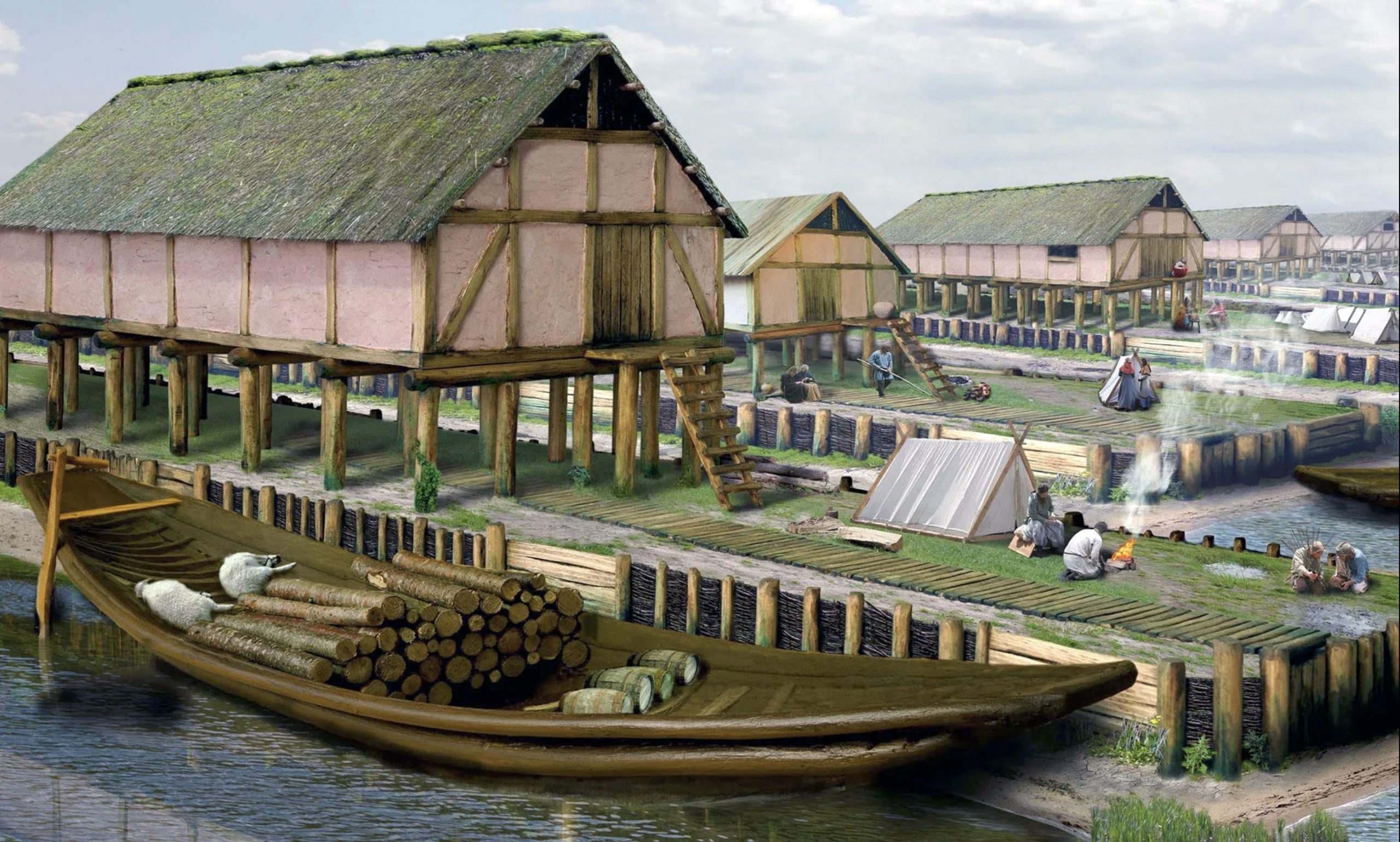
Illustration One: Early medieval trading vessel, similar to those used by Frisian merchants in the 7th-9th centuries
Based on genetic genealological data, a descendant of the lineage arrived and settled in East Anglia around 625 to 770 CE. East Anglia was an historic region in the southeastern part of the English Isle, comprising the contemporary counties of Norfolk, Suffolk, and Cambridgeshire. Historically, it was a sixth-century Anglo-Saxon kingdom, with its name deriving from the “East Angles” who predominately settled there. [9]
The Dynamic Nature of Ethnicity
Depending on which ‘lens’ of historical time we are using to look at the past (e.g. traditional genealogical time, the time of lineages or long term deep history), ethnicity is considered an imprecise analytical tool or term. [10] It is an identifier, useful to describe social and cultural groups within specific historical time perods. Even then, its qualifying labels are fluid social constructs rather than a fixed biological or genetic fact; often blending overlapping, shifting, and subjective and material factors like culture, language, ancestry, self- and group-identification.
Ethnicity is an achieved as well as an ascribed social attribute. Its meaning and significance depends on which group or person is using the term for their identity or for identifying ‘other’s’ identities. It is a social construct that can be used to differentiate social relations, power relationships and create and reinforce cultural distinctions. [11]
Unlike terms associated with strict classification systems, ethnicity is dynamic. It varies across time, geography, and personal experience. While often conflated with genetic ancestry, ethnicity is learned, socially based and cultural, not inherited through DNA. Scientific research shows more genetic variation within ethnic groups than between them, making it a poor discriminating tool. [12]
Welsh culture began to emerge following the Roman withdrawal from Britain in the fifth century, with a distinct identity taking shape among the Celtic Britons by the sixth century. The culture coalesced as these Brythonic-speaking people were pushed into the western peninsula, with the term “Cymry”used for self idenification, appearing by the seventh century. [13]
“By 430 a radical cultural change is evident in Britain, affecting, for example, burial styles, building styles and clothing. Both the archaeological evidence and genetic findings indicate that these changes were influenced to at least some extent by immigrants who were coming from the North Sea coasts of what is now the Netherlands, Germany and Denmark, but some of the changes also have parallels with northern Gaul, which was similarly a country where Roman forces and government were weakening or being withdrawn. Usage of Old English cannot be proven during this period, but its closest relatives were the Old Frisian and Old Saxon dialects of the same continental coastal regions, and so some amount of migration is once again implied.” [14]
“Sub-Roman Britannia underwent rapid change in the course of fifty years between AD 550-600. At the start of this period, the Angle and Saxon kingdoms on the east and south coasts were firmly established. Many of the rapidly-formed Romano-British territories in those areas had been swept away in the late fifth century. A few were managing to hold out, but they were becoming increasingly surrounded and squeezed by encroaching invaders.” [15]
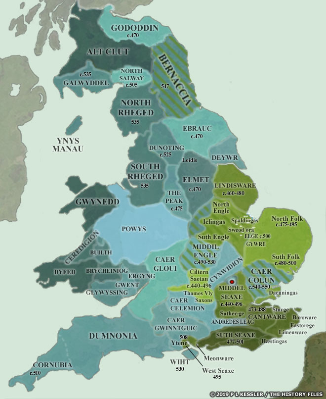
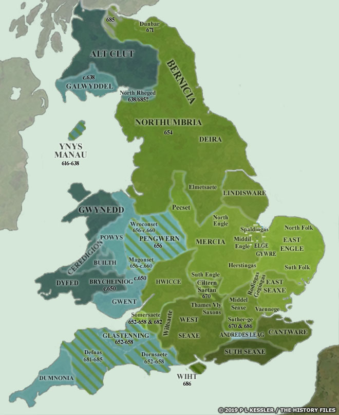
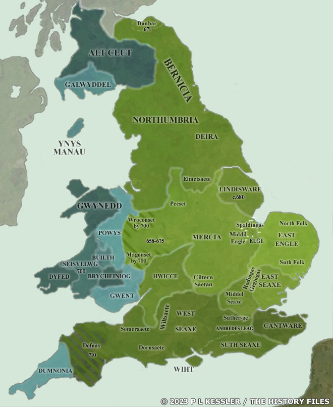
Political and ethnic boundaries in England between 400–800 CE were loosely correlated but rarely identical: political lines shifted rapidly, while ethnic and social identities were situational, layered, and often cross‑cut those frontiers (see illustration two). [16]
Illustration Two: Sequential Maps of Anglo-Saxon Conquest 450 – 700 CE [17]
After the end of Roman rule, power fragmented into small Romano‑British polities and warbands rather than clearly bounded “states” or “kingdoms”, and their authority faded unevenly across regions. Anglo‑Saxon groups (Angles, Saxons, Jutes, to a lesser extrent Frisians, etc.) arrived as federate troops and migrants into this landscape, gradually carving out lordships that hardened into early kingdoms, especially in the east and southeast. In this early phase “Britons” and “Saxons” function more as oppositional, ‘rhetorical groups in historic texts‘ illustrated in written accounts, such as those of the monk Gildas [18], rather than as stable, self‑ascribed ethnic communities mapped cleanly onto territories. Archaeology and historical studies suggest considerable local continuity of late Roman populations beneath these new ethnic political labels, complicating any simple ethnic replacement model (see illustration three). [19]
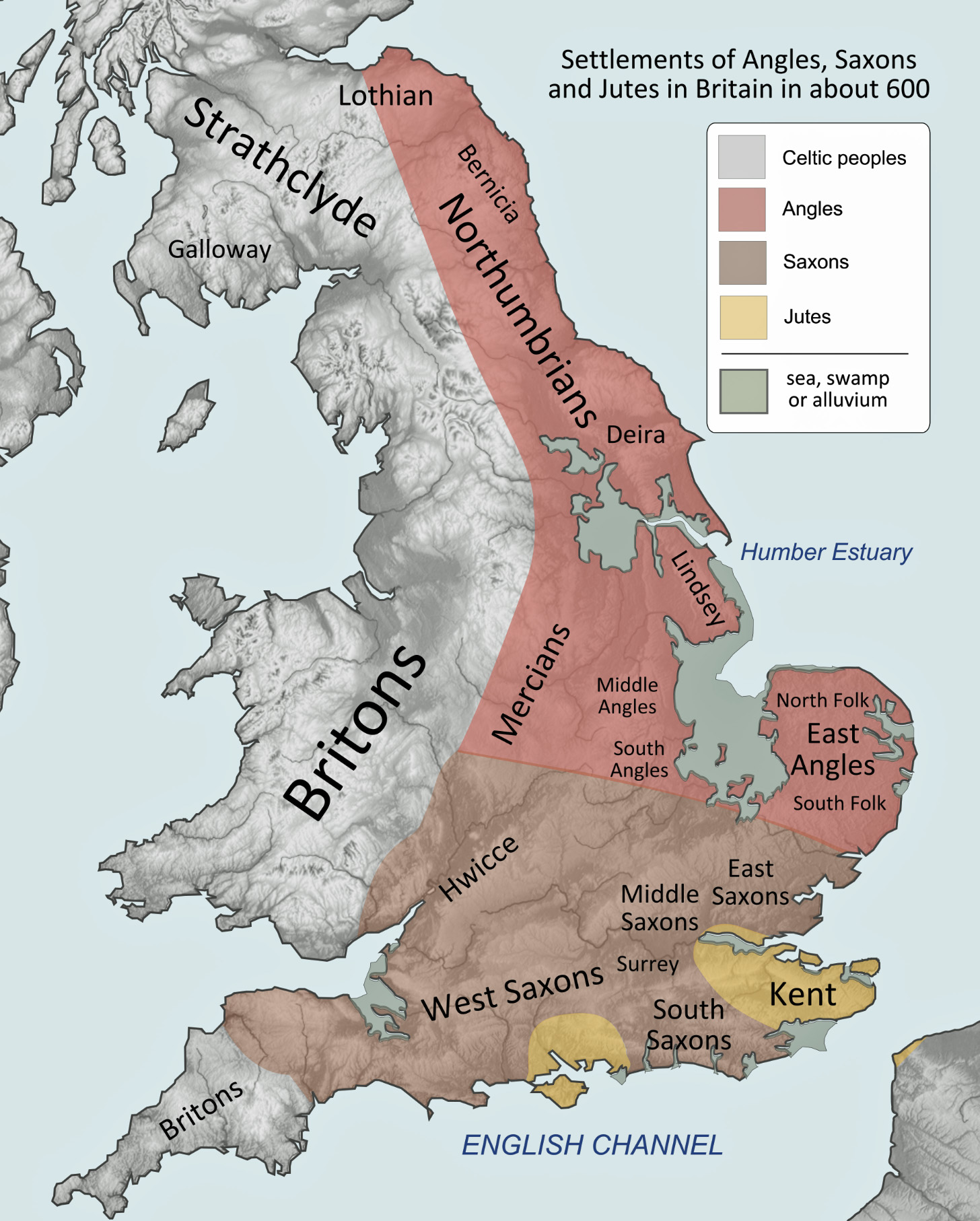
Illustration Three: Settlements of Angles, Saxons and Jutes Circa 600 CE
By the later sixth–seventh centuries, larger kingdoms (Northumbria, Mercia, Kent, Wessex, East Anglia, Sussex, Essex) emerged, but their boundaries remained fluid zones of overlordship, tribute, and shifting alliances rather than fixed lines. Within any one kingdom, elites might cultivate an “Anglo‑Saxon” royal identity, while subject communities could be Brittonic‑speaking, mixed, or only loosely integrated into royal structures. Political expansion (for example, Mercian pressure on Welsh polities or Wessex’s moves into Sussex, Surrey, and Kent) routinely brought people of different linguistic and cultural backgrounds under one crown without instant assimilation. Ethnic designations in narrative historical sources tend to appear at precisely these points of contest, where authors use labels (for example, Saxones, Brittones, etc.) polemically to mark insiders and outsiders. [20]
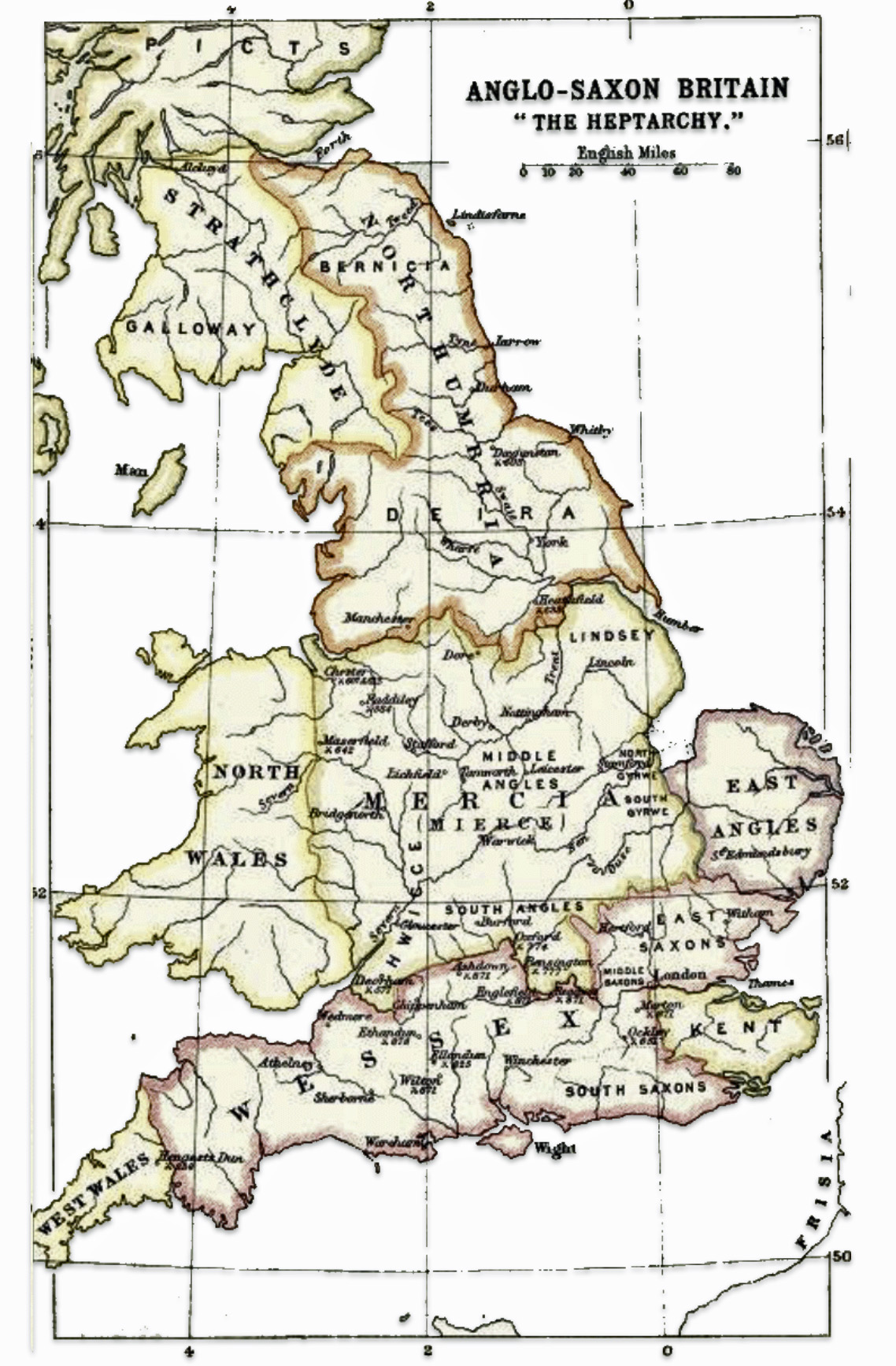
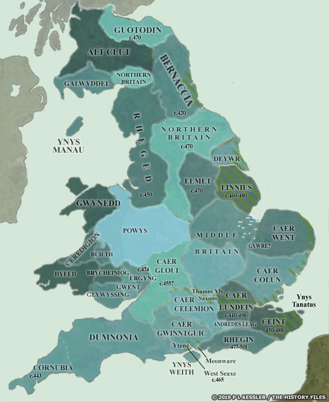
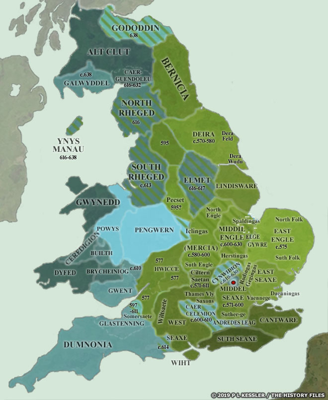
Around 600 CE, seven principal kingdoms had emerged, beginning the so-called period of the Heptarchy. The Heptarchy was the division of Anglo-Saxon England between the sixth and eighth centuries into petty kingdoms, conventionally referring to the seven kingdoms of East Anglia, Essex, Kent, Mercia, Northumbria, Sussex, and Wessex. The period of petty kingdoms came to an end in the eighth century, when England was divided into the four dominant kingdoms of East Anglia, Mercia, Northumbria, and Wessex. [21]
Illustration Four: The Heptarchy
As some kingdoms achieved temporary hegemony (e.g. Northumbria in the seventh century, Mercia in the eighth), political success provided a platform to project certain ethnic and origin myths (e.g. royal genealogies from Woden) across wider areas. [22] Yet modern analyses argue that ethnic identity in this period is best seen as a situational construct: origin myths, law, and language could be emphasized or downplayed depending on context, especially in court politics and diplomacy. This means that when political frontiers shifted, the salience of particular ethnic labels often shifted with them, rather than ethnic “groups” moving as cohesive, bounded units. [23]
By 800 CE, the political landscape shows larger, more coherent kingdoms. Ethnic identities in Britain before 700–800 CE were not clearly defined or straightforwardly assigned; they crystallized gradually, with “English”, “Welsh” or “Scottish” identity only becoming a meaningful, wider category in the later eighth–ninth centuries. Overall, the interplay can be described as one where shifting, negotiated social group hegemonies provided occasions for ethnic labels to emerge and be utilized or mobilized, but everyday ‘social belonging’ remained highly local, mixed, and context‑dependent. [24]
While the Griff(is)(es)(ith) YDNA ancestors in the 1600s may have had a ‘Welsh’ identity, their male ancestors were Frisian or Frankish migrants that initially settled in the southeastern areas of the island as part of a larger, sustained wave of Anglo-Saxon migrants coming from the northwestern contnental coastline between roughly the tail end of the 600’s CE to the mid 700’s CE. Along the eastern shore, migratory groups of new Angle and Saxon arrivals were settling in areas that were former Roman laeti settlements, asserting their geographical and cultural influence.
“Laeti, the plural form of laetus, was a term used in the late Roman Empire to denote communities of barbari (“barbarians”), i.e. foreigners, or people from outside the Empire, permitted to settle on, and granted land in, imperial territory on condition that they provide recruits for the Roman military.” [25]
By the time the YDNA genetic lineage of our family arrived on the eastern shore of the island, the fall of the last sub-Roman territories was over. The remaining unconquered kingdoms in the west, an area which was becoming known as Wales, were beginning the process of unification.
Illustration Five: Estimated Migratory Path Between Haplogroup G-Y38335 and G-Y132505
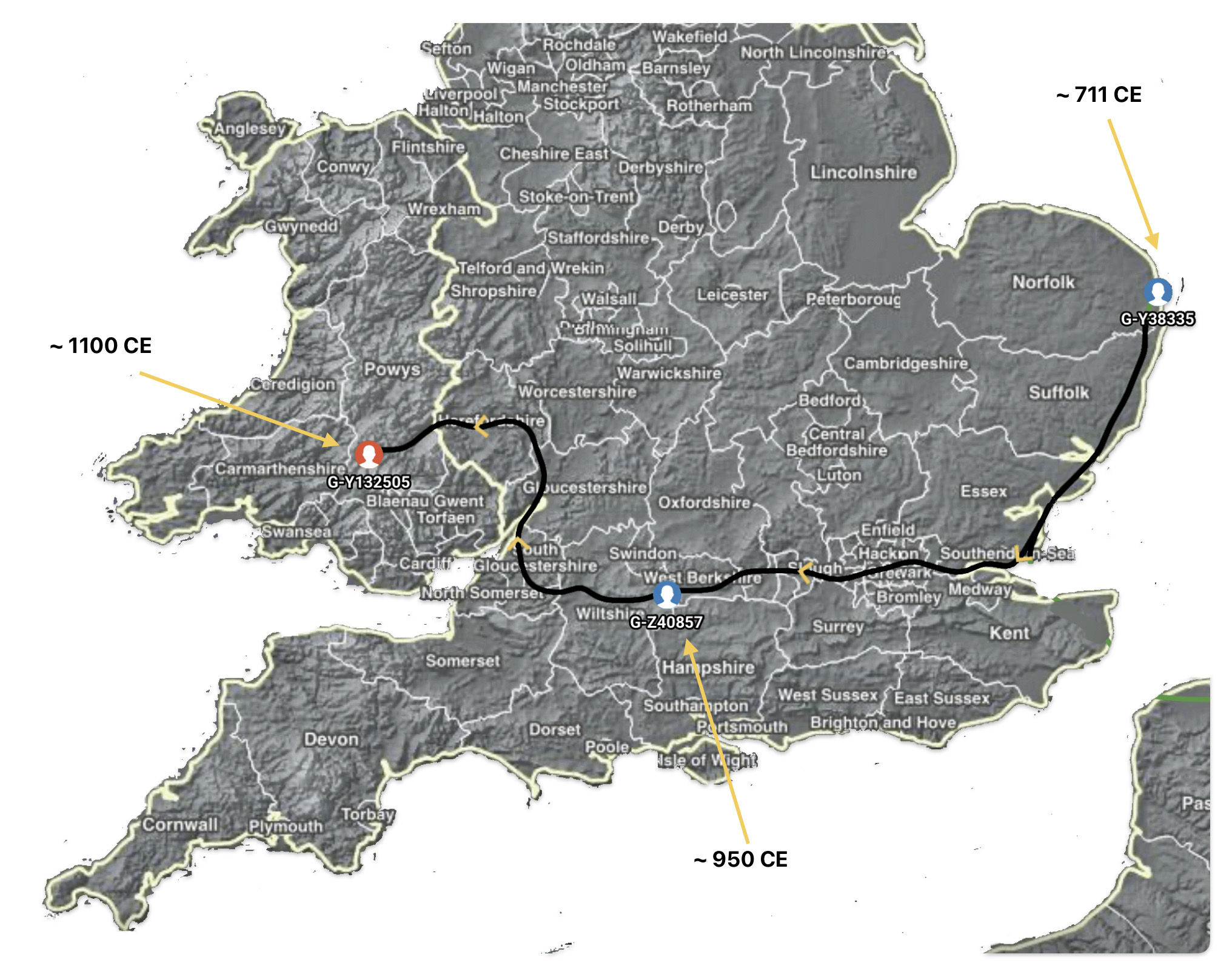
Subsequent generations of the family YDNA lineage migrated from the eastern shore westward, across the lower portion of the island, eventually locating in areas on the western peninsula around 1100 CE, each generation shifting their ‘ethnic’ group identities along the way (see illustration five above).
The Most Recent Common Ancestor of Haplogroup G-Y38335
As indicated in a previous story, the most recent common ancestor (MRCA) of haplogroup G-Z6748 may have been born around 668 CE. It is estimated that he had a 68 percent chance of being born between 525 CE and 800 CE. Another significant fact associated with this MRCA ancestor of Haplogroup G-Z6748 is that he was the last documented ancestor of the paternal line to have lived on the European mainland.
As indicated in previous stories, the genetic ancestors of the MRCA of G-Z6748 migrated through the Roman Limes area, an area that is modern day Netherlands, around the collapse of the Roman Empire, at a time and place that became increasingly controlled by Frankish groups. These ancestors continued to move northward into areas inhabited by social groups known or identified as Frisians. It is estimated that the most recent common ancestor of G-Z6748 may have lived in the Texal Island area. [26]
Illustration Six: Scientific Details of MRCA of G-Y38335
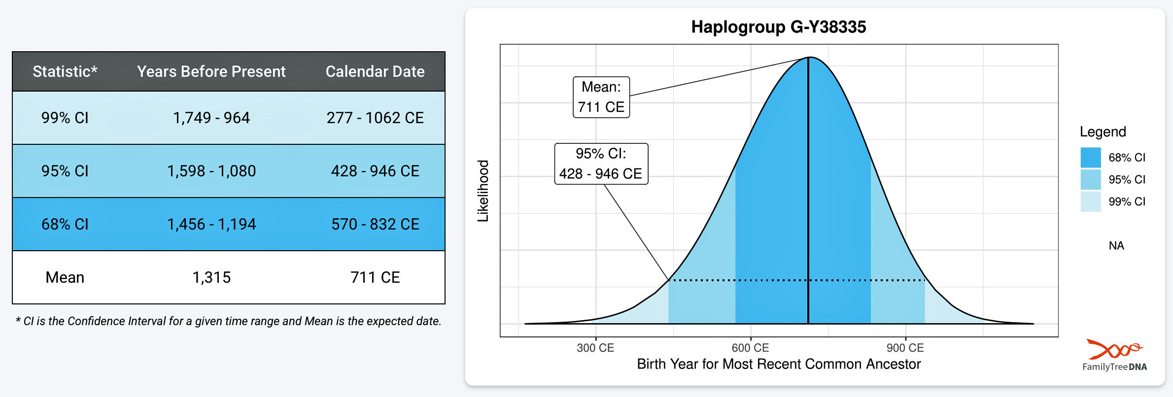
The next documented YDNA haplogroup that is associated with a common ancestor in the lineage is G-Y38335 (see illustration six). This is presumed to be the first YDNA ancestor known to have lived on what is now called the British Isle. It is estimated that this ancestor was born around 711 CE. This ancestor could have conceivably been the child, grandchild or close descendent of the most recent common ancestor of G-Z6748. This individual had a 68 percent chance of being born between 570 and 832 CE. While this roughly 265 time span is relatively short, representing about eight or nine generations of chronological time, it is a period that witnessed noteworthy changes on both sides of the ‘Oceanus Germanicus‘ and the ‘Narrow Sea‘. [27]
A comparison of the scientific details between the ancestors associated with each of the these haplogroups indicate their relative closeness in chronological order (see illustration seven below). There is only roughly 43 years between the median birth years for each ancestor. The estimates related to their dates of birth suggest they may have been only one or two generations apart. [28]
Illustration Seven: the MRCAs of G-Z6748 and G-Y38335
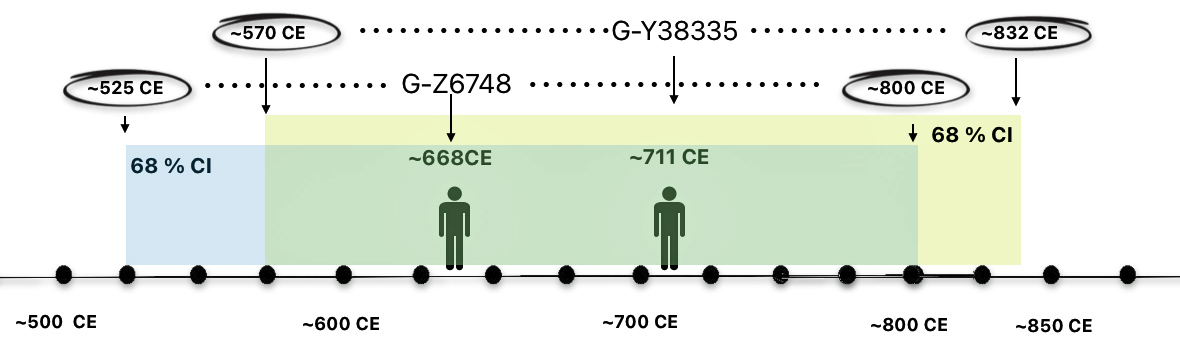
To put 43 years in historical context, in 700 CE during the Early Middle Ages, the estimated average life expectancy at birth for males in the region that is now the Netherlands was very low, likely in the mid-30s (approximately 30–35 years). This low number does not mean that men typically died in their thirties; rather, it was driven by extremely high infant and child mortality rates. Early medieval life in the region was characterized by high risks from disease, malnutrition, and, for elite males, violence, which kept the overall average low. If a male survived the dangerous years of childhood (often to age 10 or 15), his life expectancy would increase significantly, often to 50 or 60 years. Data from seventh-century European populations indicates that while life expectancy at birth was low, many adults who survived early life could live into their 60s or 70s. [29]
The Phylogeography of G-Z6848 and G-Y38335 through the Eyes of the Globetrekker Tool
Phylogeography is the study of how genealogical lineages are distributed across geographic space through time, using genetic data to infer the historical processes that generate patterns of variation. It explicitly links phylogenetics and population genetics with biogeography. [30] Much of my phylogeographical work on the migratory path of the family YDNA lineage relies on the results from the GlobetrekkerTM mapping tool, originally developed by FamilyTreeDNA (FTDNA) as an exclusive feature for their Big Y-DNA test customers. [31]
Illustration Eight: Migratory Path of Descendants of Haplogroup G-Z6748 and Haplogroup G-Y38335
If we look at a snapshot of a Globetrekker produced animated YDNA migratory path between most recent common ancestors of haplogroups G-Z6748 and G-Y38335, the migratory path of the decendants of haplogroup G-Z6748 starts on or around the Texal Island on the northwest coast (see illustration eight). This was an area inhabited by Frisian social groups when the most recent common ancestor associated with haplogroup G-Z6748 lived. [32] The migratory path hugs the western coast and then crosses the ‘narrow sea’ or what is now known as the English Channel. [33] The path then proceeds northward along the coast of the English Isle to an area on the coast line that is presently part of the county of Norfolk or Suffolk. From there, the migratory path returns southward along the cost and then heads westward towards the western peninsula of the English Isle.
Globetrekker uses a landscape-based least‑cost path model, not a “shortest straight line” model, so its algorithm strongly prefers hugging coasts and land over open‑sea crossings. [34] It first estimates a coordinate for each haplogroup by averaging locations of testers and ancient samples, then “snaps” any point that falls in the sea back onto nearby land. Once those points are fixed, it connects them with Least Cost Paths (LCPs), which try to find the easiest route between points, not the geometrically shortest route. [35]
The algorithm assigns high “costs” to certain environments:
- Open ocean is weighted as much more costly than land.
- Coastal waters within about 200 km of land are less costly, and the model prefers routes that minimize offshore distance.
- Steep slopes and strong adverse currents also add cost. [36]
Because open sea is heavily ‘penalized’, the least‑cost solution typically follows coastlines (Texel down the Dutch coast, along the Channel, then up to Norfolk) instead of a direct sea crossing, even if a straight ‘ship‑like line’ would be shorter on a modern map or perhaps make historic sense.
So the Texel‑to‑Norfolk path you see in illustration four is not claiming that the ancestral migratory path literally followed the entire coastline. It is simply the model’s best‑fit “easy terrain” corridor linking two inferred haplogroup locations under assumptions that people stayed close to land, avoided long open‑water stretches, and moved within the ‘LGM‑style’ coastline. For historical periods when direct boat crossings were common, that coastal path is better read as a ‘broad migratory corridor‘ rather than a literal route choice.
FamilyTreeDNA has not publicly documented specific justifications for placing the most recent comon ancestor of haplogroup G‑Y38335 in the modern day Norwich/east Norfolk coastal area. The estimated location of this ancestor is perhaps driven by a general algorithm that combines the geographic distribution of the self reported dates and places of “earliest known ancestors” of modern FamilyTreeDNA Big Y testers, any associated ancient Y‑DNA samples, and the positions of downstream branches of the YDNA‑tree.
A Sea Centered Approach Toward Migration
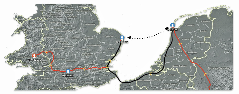
During the time when each of these ancestors lived, a direct sea crossing between the Frisian coast (including Texel) and the East Anglian coast was more realistic than a laborious “coastal terrestrial” route. During this time perod, a mature maritime contact zone existed between the Frisian coast and the coast of Britanniae Major. [37] Based on historical and archeaological evidence, it is more realistic to predict a migratory path via sea from the Frisian coast areas of the continent to the eastern coast of the British Isle as depicted by the dotted line in illustration nine below. [38]
Illustration Nine: Alternative Migratory Path
A number of scholars studying the early medieval Britain and the North Sea coastal world have utilized a “sea ‑ centered” or maritime‑ landscape approach in understanding this time period and geographical region. This body of research highlights the influence of:
(1) coastal marshes, estuaries, and islands as densely occupied and socially distinctive environments;
(2) landing places and small ports as key interfaces; and
(3) cross‑North‑Sea and Channel connections as fundamental to group identity formation and the economy in the sixth through tenth centuries (see side bar discussion). [39]
Guided by their maritime research orientation, their analysis and survey of archaeological sites have revealed an increase in known coastal sites: small farmsteads, seasonal camps, production zones and minor landing places that were previously invisible or dismissed as marginal. This has led to archaeological research models in which early medieval coastlines (e.g. the English Channel and southern North Sea) are seen as heavily exploited, socially complex settlement belts, not thinly populated liminal, transitional, zones.
Advances in geological and geomorphological research clarified shifting shorelines, inlets, and river mouths, making it possible to relocate early medieval landing places, estuarine routes, and drowned / eroded sites, and thus to reconstruct more complex maritime network topographies. Newly found and re‑interpreted artefact finds (coins, imported pottery, lava querns, weights and scales, precious metals) demonstrate that access to imported goods in coastal regions was widespread across many types of settlements and not confined to major emporia or trading centers. [40]
Emporium (emporia – plural) is a term that has been used to describe a geographical center of heightened trade during the Early Medieval Era.

Maritime and Seascape Archaeological Perspectives
Maritime and seascape perspectives have pushed scholars to treat coasts and seas as structuring elements in their own right, which has reshaped early medieval settlement models away from land‑locked, “central place plus hinterland” schemes toward coastal networks of settlements tied together by water.
Earlier archaeological models tended to project inland “central place” hierarchies seaward, treating the coast as a marginal fringe or simple export outlet of agrarian hinterlands. Maritime and seascape perspectives map chains of landing places, wics/emporia [41] and beach markets as a network of places whose primary routes are along coasts and tidal rivers, with the sea as the main connective medium rather than an edge of inland territory (see illustration ten).
Instead of reading coastal sites as passive outlets of inland polities, these archaeological models see distinct maritime communities whose identities are shaped by seafaring, exchange, and shared coastal ecologies on both sides of the Channel and North Sea. [42]
A notable example of this approach is found in Robert Van de Noort’s North Sea Archaeologies. He argues that taking the North Sea itself as the central “place” or focal point produces a different kind of archaeology, one that foregrounds mobility, connectivity, and human–sea entanglements. His work presents a “maritime biography” of the North Sea, tracing how human engagements with this sea changed over time rather than treating the sea as a backdrop to terrestrial histories. A key aim of his work is to show what an archaeology centered on a fluid seascape looks like, in contrast to conventional land‑based regional syntheses, and how this perspective alters interpretations of past societies. The sea is treated as a culturally constituted space, not just a void between coasts. His perspective stresses seascapes, routeways, and horizons instead of political or ethnic territories. [43]
Van de Noort’s North Sea is delimited on the west by the east coast of Britain and the Scottish archipelagos of the Orkneys and the Shetlands. On the east side, the focus of Ven de Noort’s work is delimited by the coasts of Norway south of Bergen, the Bohuslän province coast of Sweden, the shores of Denmark, the north-western coasts of Germany, as well as those of the Netherlands and Belgium, with a small part of the French coast around Dunkirk (see illustration ten).
“The early medieval North Sea was not a barrier but a highway – a broad maritime road linking the communities along its shores. In the 5th through 7th centuries, a remarkable parallel development unfolded on opposite sides of this sea: in Britain, the Anglo-Saxons were forging new kingdoms, while across the water on the continent, the Frisians were shaping a society of their own. Far from being strangers, these two peoples were close kin. They spoke dialects so similar that missionaries like St. Willibrord could preach to the Frisians with little need for translation, implying Old English and Old Frisian were nearly mutually intelligible. They shared common gods, artistic styles, shipbuilding techniques, and even family ties. In essence, the Anglo-Saxons of England and the medieval Frisians of the North Sea coast were two branches of the same family tree – their paths diverged, yet they remained intrinsically connected by blood, language, and culture.” [44]
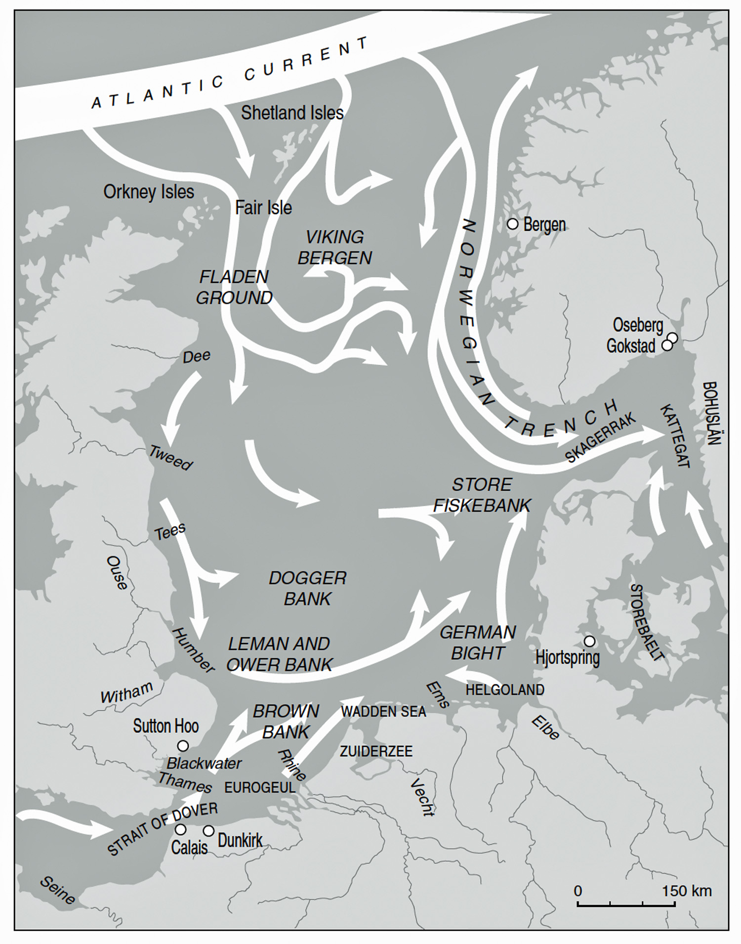
Illustration Ten: A Shared Maritime World of Atlantic and North Sea Channel Currents
Seascapes not Shorelines
Maritime and seascape archaeological studies provide key evidence for substantiating the existence of Frisian maritime networks. The research associated with this perspective substantiates patterns of movement across the North Sea through archeological findings based on coastal settlements, boat technology and trade artifacts. [45]
Within this context, early medieval Frisian population movements toward the east coast of Britain is documented less by any one “smoking gun” archaeological site and more by a body of research that treats the southern North Sea as a shared maritime world rather than a hard frontier with major trading sites. This seascape‑centered archaeological approach makes Frisian migration look like one facet of a long‑running, two‑way coastal system linking the Wadden Sea, Rhine–Meuse estuary and eastern/south‑eastern Britain.
Coastal travel and trade across the North Sea and English Channel were established long before the fifth century. As early as the third and fourth centuries, Romans reported Germanic “Saxons” raiding, and later, hired as mercenaries to defend the British coast, necessitating consistent North Sea crossings. These voyages were made in wooden ships (similar to early, oar-powered, non-sailed precursors to Viking longships). Sailors used natural cues like stellar navigation, bird flight paths, and, crucial to the North Sea, the lead line and sounding rod to measure water depth. By 600 CE, Frisian traders had developed a near-monopoly on trade in the North Sea. [46]
Key Features of Migration Period Longboats
- Clinker (Lapstrake) Construction – Overlapping planks joined with iron rivets
- Double-Ended Design – Symmetrical bow and stern for beach landing without turning
- Shallow Draft – Flat bottom for navigation in shallow waters
- Lightweight Design – Enabled portaging between waterways
- Oar Propulsion – Primary means of movement in early vessels
- Later Sail Adoption – Added by late 7th-8th centuries
- Open Hull – Undecked interior space
- Shell-First Construction – Hull built before internal framing [47]
Illustration Eleven: Migration Period Longboat
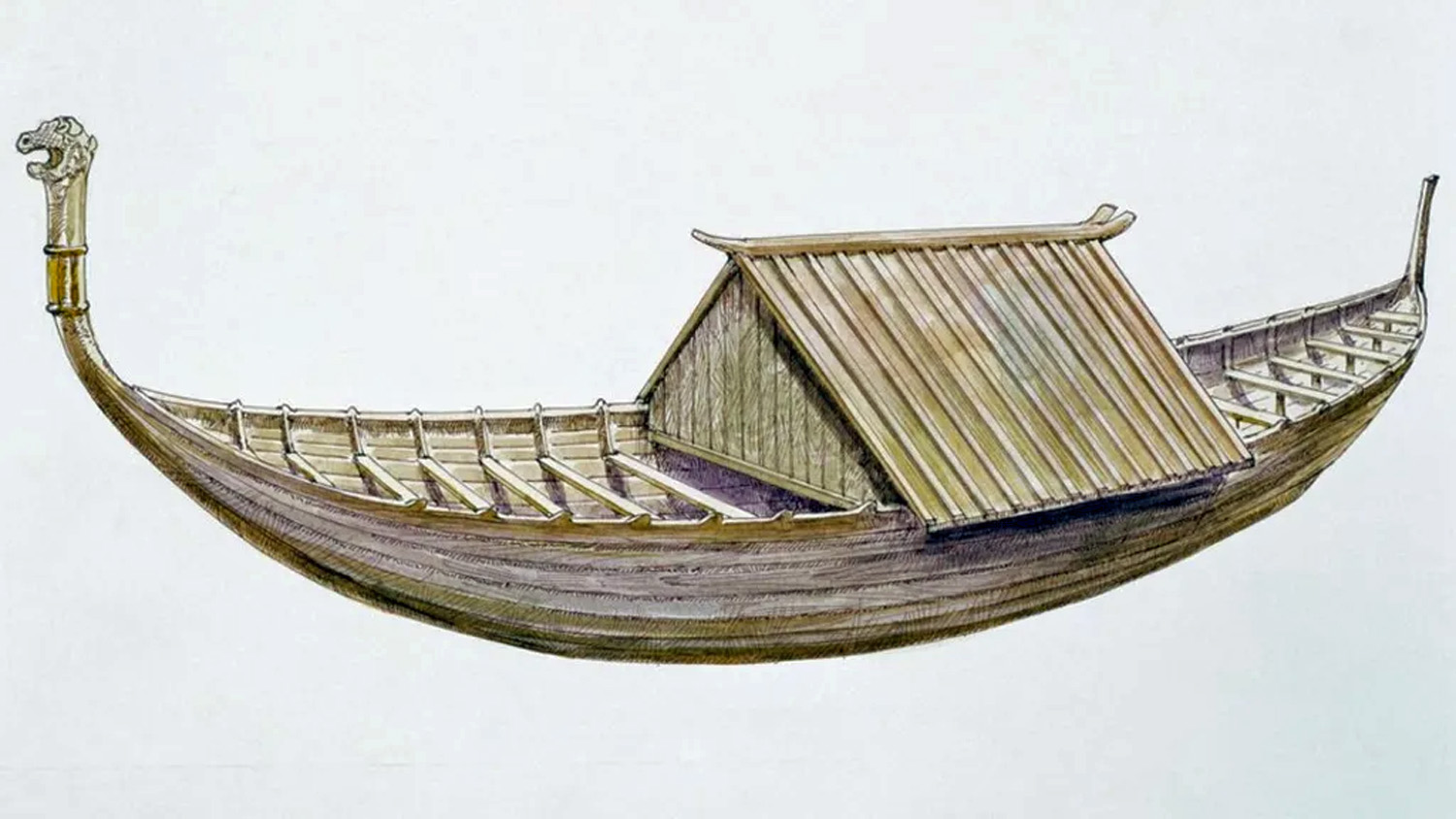
“Artist’s reconstruction of a Migration Period longboat with covered central section, showing the characteristic curved hull and high prow and stern. Such vessels were common among Frisian and Anglo-Saxon seafarers in the 5th-7th centuries, featuring clinker-built construction that would later evolve into Viking vessels.” [48]
Long‑keel, clinker‑built vessels of the broader Anglo‑Frisian and Scandinavian tradition were fully capable of open‑sea legs across the southern North Sea, as shown by ship finds, reconstructions and experimental archaeology. These vessels underpinned both the earlier Anglo‑Saxon migrations (fifth though sixth centuries) and the later Frisian trading system, indicating that open‑water crossings in this corridor were standard practice when the descendants of haplogroups G-Z6748 and G-Y38335 lived (see illustration eleven).
“The clinker-type craft, especially those constructed in the Nordic tradition, were particularly strong and suited to seafaring. They were used for trade and exchange, and the ascendancy of the Frisians in the sixth century is attributed to their prowess in sailing such boats in the waters of the North Sea.
“It seems reasonable to suggest, albeit in the absence of direct evidence, that the migrations of the post-Roman era were only possible due to the existence of reliable seafaring boats, which allowed for the movement of families with their possessions.” [49]
A Sheltered Sea Corridor
The maritime and seascape archaeological research for the North Sea reconstructs the North Sea basin as an historically contingent landscape in its own right, shaped by Holocene era sea‑level rise, estuary formation, salt‑marsh belts and reclaimed wetlands. This archaeological approach shows that by the early medieval period, the Humber–Southern Jutland corridor framed a broad, relatively “sheltered inner sea” with predictable crossings, tidal rivers as access routes, and sand‑island/terp zones on both Frisian and English sides (see illustration twelve). [50]
Illustration Twelve Britain 400–500: Anglo-Saxon Homelands and Settlements
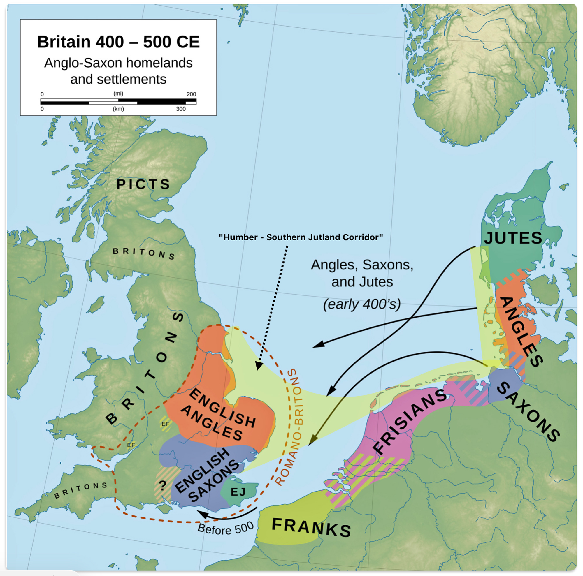
For early medieval studies, this sea corridor frames the main contact zone between eastern England, Frisia/Flanders and Denmark: Humber‑side landing places and York on one end, the Rhine–Meuse–Scheldt and Wadden harbors in the middle, and the Jutland/Schleswig ports such as Ribe on the other. It is a sea corridor that linked estuaries, wetlands and shallow‑sea routes that structured the routine movement of Anglo‑Saxon, Frisian and Danish ships, traders and migrants during the seventh to ninth centuries. [51] When you model routes and site distributions against this reconstructed seascape, traffic between Frisia and the east/south‑east English coast appears more as short‑haul coastal sailing along familiar ecological niches rather than as exceptional long‑distance voyaging. [52]
Coastal Contact Zones
A seascape perspective highlights the existence of a commerical zone of settlement locations of varying sizes between Anglo‑Saxon England and Frisia, with Dorestad, Ribe and Wadden‑Sea ports on one side and Hamwic, Ipswich, London and York on the other. Archaeological remains at these port areas show continental ceramics (e.g. Tating ware), coin series and tools moving in volume across the North Sea. Historical written sources place Frisians at the center of long‑distance trade and social diplomatic contact. Within this network, Frisian identity becomes strongly maritime: coastal traders, ship‑owners and marshland farmers whose habitual mobility, riverine reach and commercial roles made seasonal or permanent relocation to English estuaries a routine option rather than an extraordinary migration. [53]
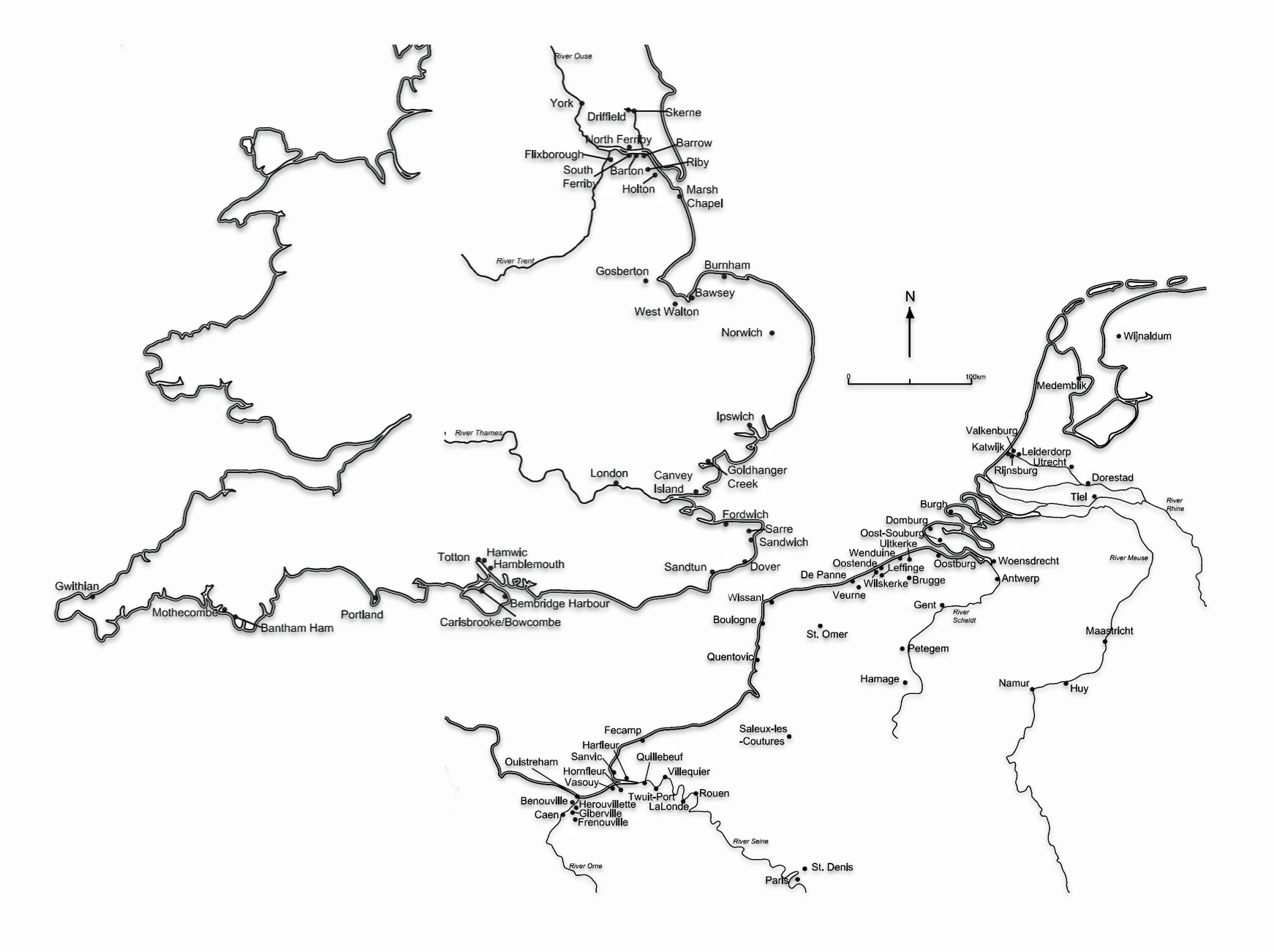
Archaeologists Loveluck and Tys argue that coastal “contact zones” along the Channel and southern North Sea were economically diverse and socially complex. Coastal access to material exchange networks shaped distinct regional identities and ‘value-systems‘ or sub-cultures. Coastal areas along the Channel and southern North Sea were not just peripheries in the commerce network but were part of a social network, integrating marine and river routes into everyday social and economic life. Coastal identities were shaped by participation in maritime networks that oftentimes cut across political boundaries, fostering shared practices and connections between opposite shores as well as between Frisians and Franks. (see illustration thirteen). [54]
“The major trading and artisan centres (often called emporia), founded on both sides of the English Channel and southern North Sea coasts, between the seventh and ninth centuries, have been interpreted as ‘ports-of-trade’ or ‘gateway communities’, controlling the redistribution of imported luxuries, surpluses and manufactured goods for kings or regional rulers. . . . (H)owever, discoveries and rediscoveries on both sides of the Channel have produced indications of a much more complex range of settlement patterns and sites of exchange than has previously been envisaged in coastal zones.” [55]
Illustration Thirteen: Location of emporia, coastal and estuarine settlements, beach/dune sites and archaeological finds/concentrations, 600 – 1000 CE
Major emporia such as Dorestad, Quentovic and Hamwic, formed only the upper tier of a broader settlement and exchange hierarchy that included small ports, landing places, and rural production sites (see illustration fourteen and fifteen). [56]
Illustration Fourteen: Coastal Settlement and Exchange Hierarchy in the Early medieval Era: Channel and Southern North Sea
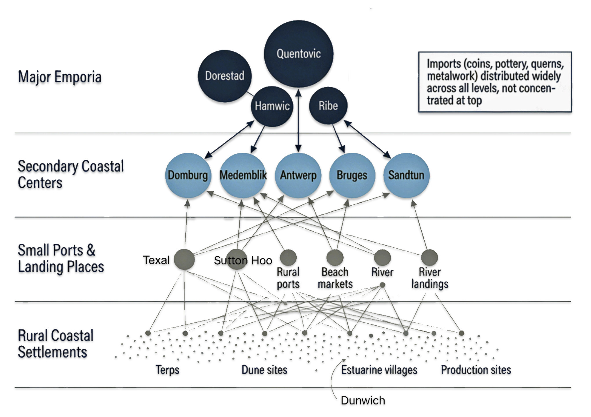
From the late seventh century a chain of specialized ports (emporia) such as Dorestad at the Rhine delta, Ribe on the Danish North Sea coast and English sites like Hamwic and Ipswich formed the core infrastructure of North Sea trade. Dorestad in particular functioned as a major shipping hub between the Frankish interior and the North Sea world, funnelling continental goods into routes toward England and Scandinavia. Textual and archaeological finds document Frisians as key operators of this system—running ships, managing market organization, and acting as brokers between hinterland producers and overseas buyers. [57]
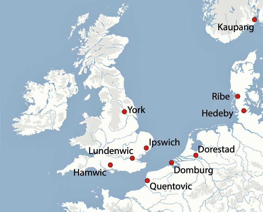
Illustration Fifteen: Major Emporia in Exchange Hierarchy
Frisian merchants in the seventh to eighth centuries handled a broad spectrum of bulk staples, raw materials, and prestige items, ranging from agricultural produce and textiles to Mediterranean luxuries and slaves. [58]
Table One: Typical Flows of Products within the North Sea Trading Network
| From Region | To Region | Main goods (archaeological attestation) |
|---|---|---|
| Rhineland / inland Francia | Frisia, England, Scandinavia | Wine in barrels, glassware, lava quern‑stones, metalwork. |
| Frisia / Rhine–Meuse–Scheldt delta | England, Francia, Scandinavia | Woollen cloth, salt, fish, amber, combs, small craft goods, redistributed Mediterranean luxuries. |
| England | Frisia and Francia | Lead and tin, raw wool, hides, slaves, some textiles. |
| Scandinavia / Baltic | Frisia, Francia | Furs, amber, walrus ivory, possibly soapstone vessels. |
A Long Tradition of Anglo-Frisian Relations Between the Coastal Areas
“The migration was not a single event but rather a complex process spanning nearly two centuries. Some Anglo-Saxon groups arrived as invited mercenaries to assist Romano-British rulers against various external threats, while others came as traders who gradually established permanent settlements. Still others arrived as conquest groups, displacing or integrating with existing populations.” [59]
The emergence of North Sea navigation and the movement of various groups during the early medieval period was not the result of a sudden social change or technological revolution but an evolution of long-standing coastal trading, mercenary activities and general migration between northern Europe and Britain. This maritime activity directly facilitated the migration of Germanic groups, primarily Angles, Saxons, and Jutes, and to a lesser extent Frisians, who began to populate Britain in significant numbers from the mid-fifth century CE, immediately following the withdrawal of Roman authority. For example, archaeological evidence of early settlements in England exist in the form of fifth-century Germanic cemeteries and settlements such as Spong Hill in Norfolk and Mucking in Essex. [60]
During the time when descendants of haplogroups G-Z6748 and G-Y38335 lived, Frisian trade networks and transport patterns between the European continent and the British island were firmly established.. The trade networks and migratory patterns were part of an expansive maritime system that linked the Rhine–Meuse–Ems delta with England, Francia, and Scandinavia, with Frisian merchants acting as key intermediaries of the North Sea world. The network was anchored in river‑mouth based emporia and coastal harbors, especially Dorestad on the lower Rhine, but also smaller Frisian trade sites on the North Frisian islands and along the Wadden Sea. These sites connected inland Frankish production zones to the wider North Sea via river routes (Rhine, Meuse, Vecht) and sea‑lanes to Britain, Flanders, the Channel coast, Jutland, and southern Scandinavia. By the later seventh and eighth centuries, this system effectively turned the North Sea, parts of the Rhineland, and the English Channel into a relatively integrated commercial space.
Dorestad (Wijk bij Duurstede) was the principal hub, growing from a modest seventh century trading place under Frisian influence into a major emporium whose heyday ran roughly from the later eighth to early ninth century (see illustration sixteen) [61] Frisian merchants maintained outposts or communities in major ports around the North Sea, including York, London, Quentovic (northern Francia), Ribe, Hedeby, Kaupang and Birka, acting as commercial intermediaries. [62] At York (Fishergate), archaeological and textual evidence points to a substantial Frisian colony engaged in trade and crafts, with imported wares reaching the city “through a Frisian medium,” and a Frisian coin (sceat) indicating contacts by 705–715 CE. [63]
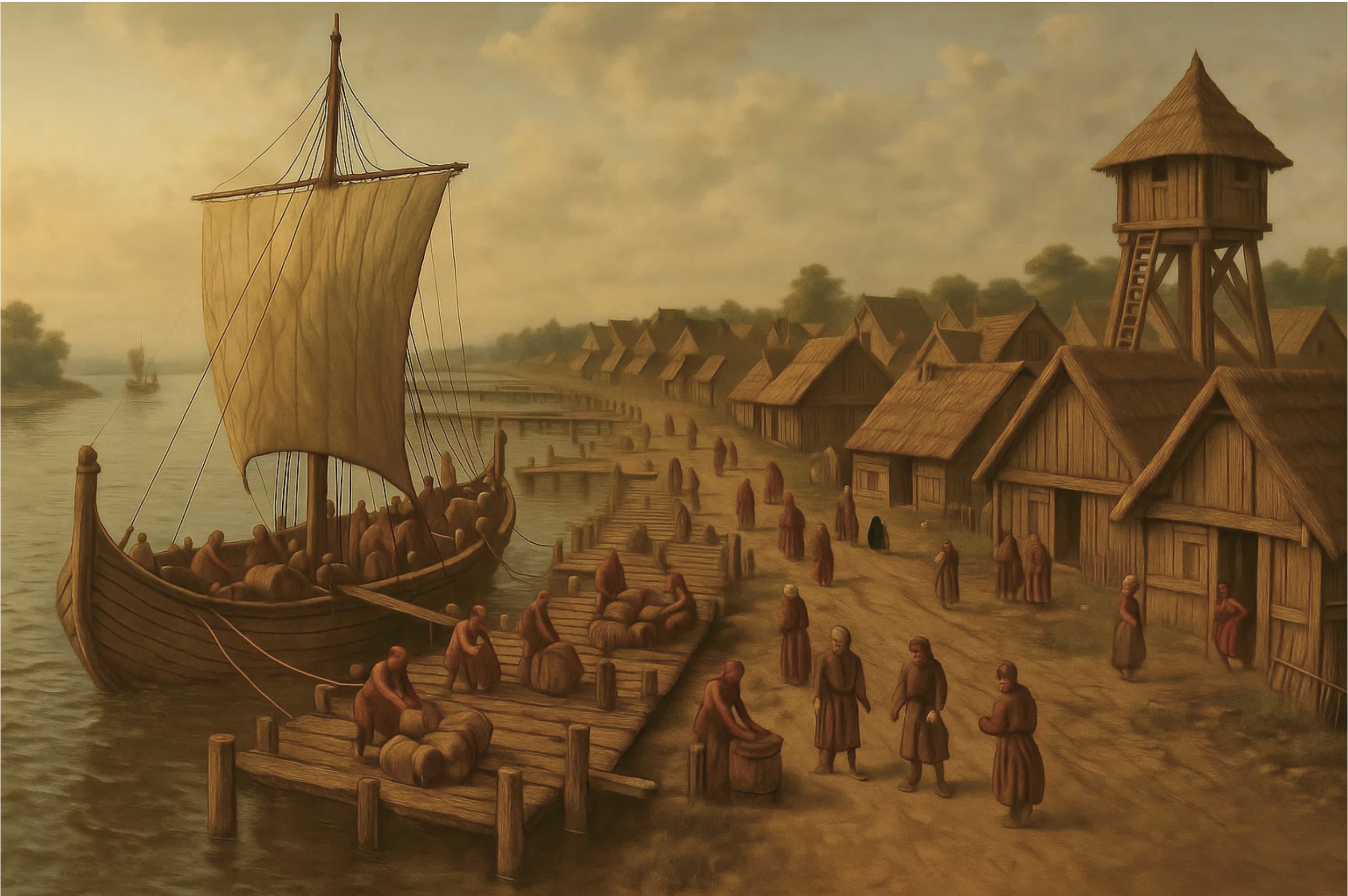
Illustration Sixteen: Artist Impression of Medieval Dorestad
Parallel Coastal Ecologies, Culture, and Settlement Signatures
Frisian scholarship emphasizes that “historical Frisia” was always defined by low‑lying marsh, tidal channels, and terp or mound‑based settlement, with repeated phases of abandonment and decolonization as sea‑level and sedimentation changed. On the English side, maritime research frameworks now stress that eastern coastal marshlands and sand islands from the Humber to the Fens and Kentish marshes were likewise densely and permanently occupied in the early medieval period, despite earlier assumptions of marginally populated areas. When you put those together, migration from Frisia to England appears as movement between structurally similar coastal ecologies: people already expert in dealing with similar environmental challenges, drainage and stock‑raising in wetland environments moving into Fenland embayments, estuary heads and marsh islands that demanded exactly the same knowledge. [64]
When archaeological sites are mapped across the whole southern North Sea seascape, cultural and technological “Anglo‑Frisian” zones emerge that straddle the water, rather than stopping at the beach. Early medieval studies point to close convergence in language and material culture between communities on both sides of the sea in the centuries after the main post-Roman Migration Period. [65] Portable objects and ceramics with shared forms appear in coastal Frisia and eastern England, and some terp reoccupations on the north continental coast in the fifth–sixth centuries show “Anglo‑Saxon” style pottery embedded within Frisian contexts, underlining how intertwined these identities became within a maritime world. Archaeological seascape approaches interpret this not as simple diffusion from one static “homeland,” but as the archaeological footprint of people circulating along sea‑lanes, intermarrying and settling in multiple harbors and marshlands. [66]
Ancestors and Descendants of G-Y38335 Migrating to East Angles
In this wider historical context, the most recent common ancestor of haplogroup G‑Z6748 who may have lived in the Texel region would have been part of a small kin-group rooted in an island–marsh environment, with everyday mobility oriented along creeks and coastal routes that easily link Texel southwards (Rhine–Meuse delta) and northwards (North Frisia, Jutland, Ribe).
By the late seventh century, the Wadden Sea and adjacent islands were part of a dense maritime cultural landscape characterized by tidal inlets, salt-marsh settlements, and natural harbors that facilitated short-haul and long-distance sailing along the North Sea coast. Texel and neighboring Wadden islands functioned as ‘nodal points’ on the sailing route between Scandinavia, Frisia and destinations such as Dorestad, making them natural staging points for voyages towards England. Archaeological work on comparable North Frisian islands and coastal marshes shows mixed farming communities with strong engagement in craft production and regional exchange, embedded in a seascape where boats, creeks, and barrier islands structured movement more than inland roads. [67]
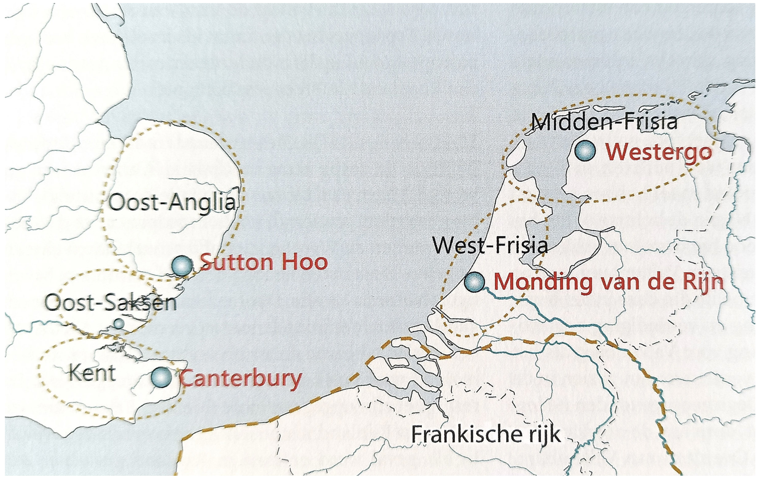
“Cultural ties between the early Anglo-Saxons and Frisians remained strong until the seventh century. Their material culture and economies were remarkably similar. They spoke closely related languages and used the same runic alphabet. Well-connected through trade, political alliances, and elite networks, their kinship is evident from archaeological finds, linguistic studies, and DNA research. By around the year 600, small Anglo-Saxon and Frisian kingdoms had emerged along both sides of the southern North Sea coast. Among these were the three Anglo-Saxon kingdoms of southern East Anglia, Essex, and eastern Kent, and the two Frisian kingdoms located at the mouth of the River Rhine and in Westergo, in the northwest of the modern Netherlands.” [68] See illustration seventeen below.
Illustration Seventeen: Kingdoms Sourrounding Southern North Sea c. 600 CE
During the period in which the descendants of G-Z6748 and G-Y38335 lived, Frisians and Anglo‑Saxons were operating extensive ship networks across the North Sea, with regular crossings rather than only coast‑hugging transport. The Frisian kingdom at its height under rulers like Aldgisl and Radbod was a maritime power whose trade and political reach depended on open‑sea routes to Anglo‑Saxon England and beyond. [69]
Texel in the seventh–ninth centuries functioned as part of the Frisian coastal island belt in the western Wadden Sea, acting as a way‑station and local harbor zone within the broader North Sea trading system. Texel was considered part of Frisia alongside islands such as Wieringen and the mainland terp regions, forming the outer, seaward margin of the Frisian coastal landscape. This ‘wider Wadden zone’ shows continuous occupation from the late Bronze/Iron Age onward, with terpen, dikes and small harbors adapted to tidal channels and salt‑marsh environments that supported both farming and seafaring.
Given this evidence, it is likely that the most recent common ancestor of G-Z6748 or one of his immediate descendants undertook a sea route from the Frisian/Wadden coast (Texel region) either directly to the East Anglia/Norfolk area or via intermediate waypoints that were part of the ‘network of coastal settlement and exchange sites‘.
Genomic analysis of early medieval burials in eastern England indicates that a large fraction of ancestry derives from populations in present-day Netherlands, northern Germany, and Denmark, consistent with sustained migration across the southern North Sea in precisely this timeframe. Many of these migrants appear not as isolated warriors but as family groups or village segments relocating along maritime corridors, which is perhaps reflective of the migratory path for common ancestors associated with G‑Z6748 and the new sub-branch G‑Y38335 after resettlement in East Anglia. [70]
The MRCA of G-Y38335 perhaps landed at of the many landing sites on the east Anglia coast (see illustration eighteen). The ancestors of G-Z6748 were possibly traders, sailors, or farmers and small-scale migrants that followed the migratory route of the Anglo, Saxon and Jutes to the eastern shores of the island. [71]
Illustration Eighteen: East Anglia
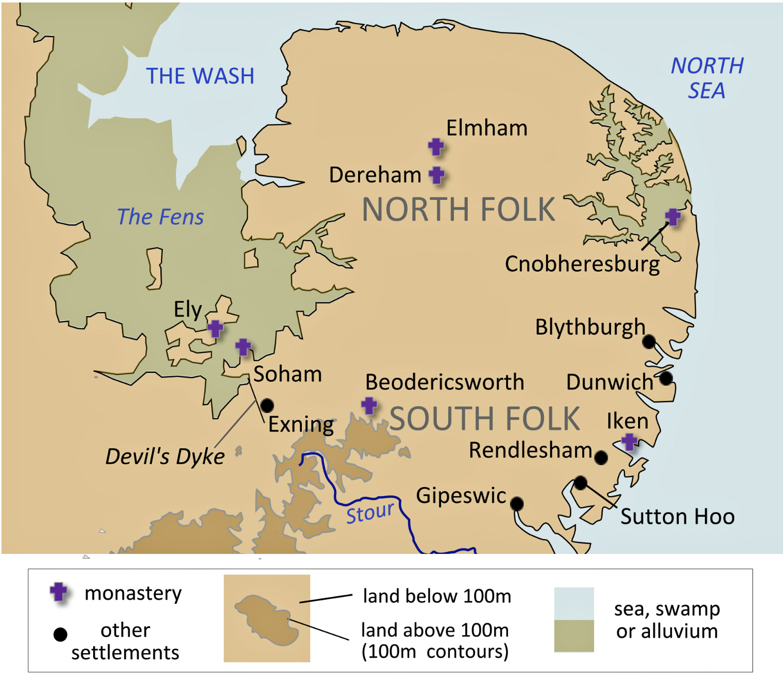
“The Anglo-Saxons settled the site of the (Norwich) some time between the 5th and 7th centuries, founding the towns of Northwic (“North Harbour”), from which Norwich takes its name, and Westwic (at Norwich-over-the-Water) and a lesser settlement at Thorpe. . . . It is possible that three separate early Anglo-Saxon settlements, one north of the river and two either side on the south, joined as they grew; or that a single Anglo-Saxon settlement, north of the river Wensum-Yare, emerged in the mid-7th century. [72]
Overall, current archaeological studies , toponymical investigations [73] and genetic work supports the view of continued, small‑scale Frisian participation in movements into eastern Britain in 700–800, embedded in a broader North Sea population flow rather than as a clearly bounded “mass Frisian migration” [74]
Early medieval narrative sources (Bede, Anglo-Saxon Chronicle) do not list Frisians among the major ethnic groups migrating to Britain. However, they were part of marginal elements of the migration movement of Angles, Saxons, and Jutes. [75] Frisians appear in English contexts from the seventh–eighth century as merchants and sailors, for example Frisian traders documented in London and a Frisian presence at York by the eighth century. [76] Hagiographical and missionary material (Willibrord, Boniface) show Anglo‑Frisian ecclesiastical and political contact across the North Sea in precisely the 690–750 window that the descendants of G-Z6748 and G-Y38335 possibly lived, which presupposes regular two‑way movement of people. [77]
Sources
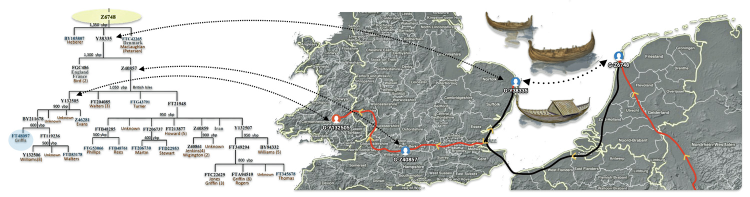
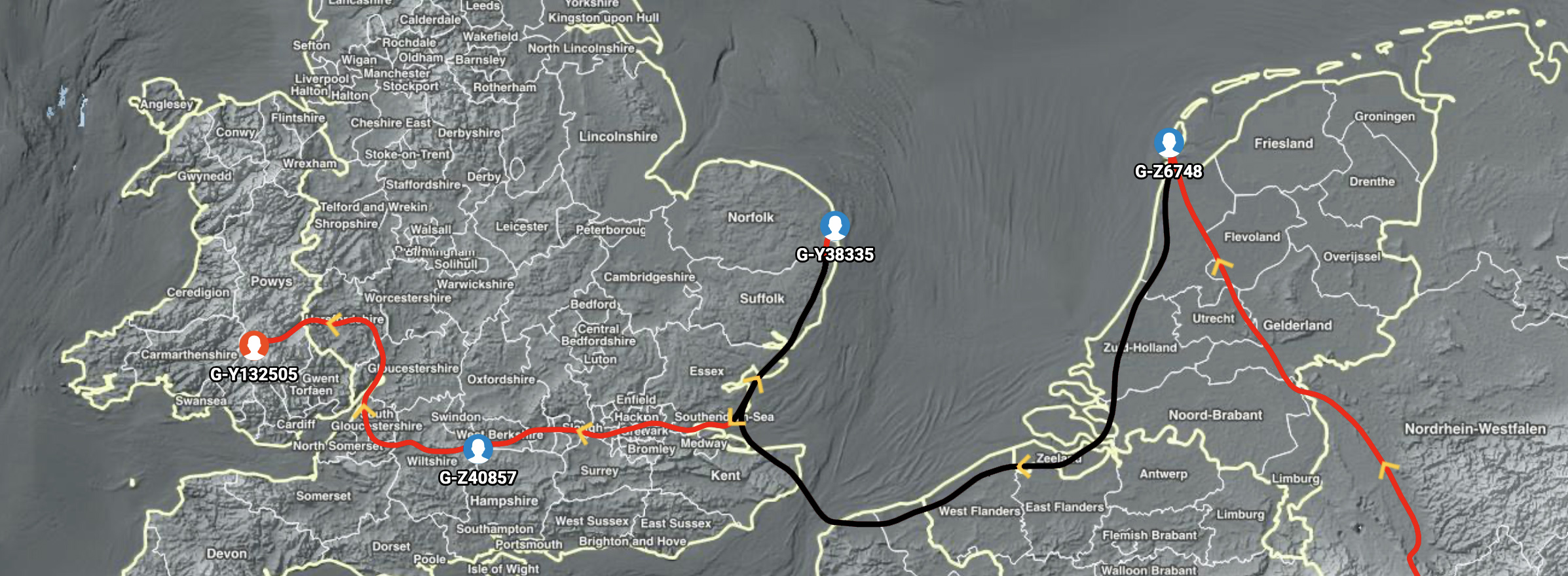
Feature Banner for the Story: On the left hand side of the banner for this story portrays the phylogenetic tree for YDNA haplogroup branches or subclades of Haplogroup G-Z6748. The right hand side is snap shot of the estimated migratory path between most recent common ancestors associated with haplogrups , G-Z6748 > G-Y38335 > G-Z40857 > G-Y132505. The dotted line from the European continent and the British Isle represents an alternative route that YDNA descendants may have taken.
[1]The most recent publically recognized haplogroup for the YDNA lineage is G-BY211678. There is insufficient information to estimate the location of the most recent common ancestor asociated with haplogroup G-BY211678. The geographical location of the preceding haplogroup, G-Y132505, is estimated to be in an area currently known as Wales. Hence, the YDNA lineage is estimated to have been in the Wales since 1100 CE.
Recent YDNA Lineage for G-Y211678
| Haplogroup | Age Estimate | Years before Prior Haplogroup | Immediate Descendants | Number of Testd Modern Descendants |
|---|---|---|---|---|
| Haplogroup | Age Estimate | Time Passed | Immediate Descendants | Tested Modern Descendants |
| G-BY211678 | 1400 CE | 300 years | 2 | 11 |
| G-Y132505 | 1100 C | 150 years | 4 | 14 |
| G-Z40857 | 950 CE | 250 years | 4 | 60 |
| G-Y38335 | 700 CE | <100 years | 2 | 62 |
| G-Z6748 | 650 CE | 2,850 years | 2 | 153 |
[2] The Romans officially left England around AD 410, when Emperor Honorius told the Britons to “look to their own defences” as the Empire faced collapse. While 410 is the accepted date for the end of formal Roman administration and the withdrawal of legions, Roman cultural influence and some aspects of Roman-British life declined gradually over the following decades. The withdrawal led to the collapse of the Roman economy, with towns shrinking and coin usage becoming rare by AD 425.
Roman Britain, Wikipedia, This page was last edited on 9 February 2026, https://en.wikipedia.org/wiki/Roman_Britain
[3] Anglo-Saxon settlement of Britain, Wikipedia, This page was last edited on 19 February 2026, https://en.wikipedia.org/wiki/Anglo-Saxon_settlement_of_Britain
[4] History of Anglo-Saxon England, Wikipedia, This page was last edited on 19 February 2026, https://en.wikipedia.org/wiki/History_of_Anglo-Saxon_England
Hills, Catherine, The Anglo-Saxon invasion and the beginnings of the ‘English’, Early & Medieval Migrations AD 43 -1500, https://www.ourmigrationstory.org.uk/oms/anglo-saxon-migrations
Nicolay, J. Settlement research and material culture in the northern Netherlands. Groningen: Barkhuis, 2010
[5] Wales in the Early Middle Ages, Wikipedia, This page was last edited on 23 November 2025, https://en.wikipedia.org/wiki/Wales_in_the_Early_Middle_Ages
Cymru, Wikipedia, This page was last edited on 15 March 2026, https://en.wikipedia.org/wiki/Cymru
Welsh People, Wikipedia, This page was last edited on 21 March 2026, https://en.wikipedia.org/wiki/Welsh_people
Etymology of Wales, Wikipedia, This page was last edited on 30 October 2025, https://en.wikipedia.org/wiki/Etymology_of_Wales
Gruffudd, Pyrs, Carter, Harold, Smith, J(enkyn) Beverley. “Wales”. Encyclopedia Britannica, 26 Mar. 2026, https://www.britannica.com/place/Wales . Accessed 2 March 2026.
Principality of Wales, Wikipedia, This page was last edited on 9 March 2026, https://en.wikipedia.org/wiki/Principality_of_Wales
[6] Wales in the Early Middle Ages, Wikipedia, This page was last edited on 23 November 2025, https://en.wikipedia.org/wiki/Wales_in_the_Early_Middle_Ages
Principality of Wales, Wikipedia, This page was last edited on 9 March 2026, https://en.wikipedia.org/wiki/Principality_of_Wales
[7] Principality of Wales, Wikipedia, This page was last edited on 9 March 2026, https://en.wikipedia.org/wiki/Principality_of_Wales
[8] History of Anglo-Saxon England, Wikipedia, This page was last edited on 8 March 2026, https://en.wikipedia.org/wiki/History_of_Anglo-Saxon_England
[9] East Anglia, Wikipedia, This page was last edited on 18 February 2026, https://en.wikipedia.org/wiki/East_Anglia
Kingdom of East Anglia, Wikipedia, This page was last edited on 12 February 2026, https://en.wikipedia.org/wiki/Kingdom_of_East_Anglia
Britannica Editors. “East Anglia”. Encyclopedia Britannica, 29 Jan. 2026, https://www.britannica.com/place/East-Anglia
[10] See the following stories:
Jim Griffis, Different Layers of Genealogical Time – Part One , January 4, 2025, Griffis Family Selected Stories from the Past, https://griffis.org/different-layers-of-genealogical-time-part-one/
Jim Griffis, Weaving Facts into a Family Story in Different Layers of Genealogical Time : Part Two January 31, 2025, Griffis Family Selected Stories from the Past, https://griffis.org/weaving-facts-into-a-family-story-in-different-layers-of-genealogical-time-part-two/
Jim Griffis, The Orientation of Family Narratives Across Time Layers : Part Three , February 28, 2025, Griffis Family Selected Stories from the Past, https://griffis.org/the-orientation-of-family-narratives-across-time-layers-part-three/
[11] See: Jim Griffis, The Use of Terms “Ethnicity” and “Tribe” to Describe the Complexity and Fluidity of Groups Across the Late Prehistory and Early Historical Periods, November 30, 2025, Griffis Family, Selected Stories from the Past, https://griffis.org/the-use-of-the-terms-ethnicity-and-tribe/
[12] Scientific research consistently confirms that approximately 85-95 percent of human genetic variation exists within ethnic or population groups, while only 5-15 percent lies between them. This indicates that any two individuals from the same population are often as genetically different from each other as they are from someone in a different population, undermining the biological basis for rigid racial categories.
Duello TM, Rivedal S, Wickland C, Weller A. Race and genetics versus ‘race’ in genetics: A systematic review of the use of African ancestry in genetic studies. Evol Med Public Health. 2021 Jun 15;9(1):232-245. doi: 10.1093/emph/eoab018. Erratum in: Evol Med Public Health. 2021 Oct 27;9(1):289-291. doi: 10.1093/emph/eoab025. PMID: 34815885; PMCID: PMC8604262. https://pmc.ncbi.nlm.nih.gov/articles/PMC8604262/
Graham , Sarah, Genetic Study Reveals Similarities between Diverse Populations, 20 Dec 2002, Scientific American, https://www.scientificamerican.com/article/genetic-study-reveals-sim/
[13] Key aspects of the emergence of Welsh culture include:
- Early Development (fifth–seventh century): After 410 AD, Romano-British populations in the west established independent kingdoms, creating a distinct culture separate from the Anglo-Saxon invaders.
- Language Evolution: “Primitive Welsh” developed between 550 and 800 AD, separating from other Brythonic languages.
- Emergence of “Cymry” (c. 633 CE): The people began calling themselves Cymry (compatriots), the country Cymru (Wales), and their language Cymraeg by the early seventh century.
- Cultural Identity (twelfth century): Historians generally agree that a strong, unified sense of Welsh identity was firmly in place by the twelfth century.
- Cultural Traditions: Early forms of poetry and literature were central to this emerging identity, with traditions having roots tracing back to this medieval period.
While regional kingdoms like Gwynedd and Powys existed earlier, a collective Welsh national consciousness grew in response to the need to defend their land, language, and customs.
Culture of Wales, Wikipedia, This page was last edited on 12 January 2026, https://en.wikipedia.org/wiki/Culture_of_Wales
History of the Welsh language, Wikipedia, This page was last edited on 23 December 2025, https://en.wikipedia.org/wiki/History_of_the_Welsh_language
Welsh Language, Wikipedia, This page was last edited on 2 February 2026, https://en.wikipedia.org/wiki/Welsh_language
History of Wales, Wikipedia, This page was last edited on 10 January 2026, https://en.wikipedia.org/wiki/History_of_Wales
Wales in the Early Middle Ages, Wikipedia, This page was last edited on 23 November 2025, https://en.wikipedia.org/wiki/Wales_in_the_Early_Middle_Ages
[14] End of Roman era and Anglo-Saxon origins, History of Anglo-Saxon England, Wikipedia, This page was last edited on 19 February 2026, https://en.wikipedia.org/wiki/History_of_Anglo-Saxon_England
[15] P.L. Kessler, Map of Anglo-Saxon Conquest Britain AD 550-600, The History Files, 2023, https://www.historyfiles.co.uk/FeaturesBritain/BritishMapAD550.htm
[16] Limmer, Michael Sean, TRhe Transformation of Identity in Early Medieval England: Continuity, Disruption, and Creolization, MA Thesis, University of New Mexico, Jul 2021, https://digitalrepository.unm.edu/cgi/viewcontent.cgi?article=1299&context=hist_etds
History of Anglo-Saxon England, Wikipedia, This page was last edited on 8 March 2026, https://en.wikipedia.org/wiki/History_of_Anglo-Saxon_England
Harland, James M., Rethinking Ethnicity and ›Otherness‹ in Early Anglo-Saxon England, medieval worlds, No. 5 , 2017, 113-142, https://medievalworlds.net/0xc1aa5572%200x00369e4f.pdf
Geary, Patrick J. , Ethnic identity as a situational construct in the early middle ages*), Mitteilungen der Anthropologischen Gesellschaft in Wien (MAGW) Band 113, 1983, S. 15-26, https://albert.ias.edu/server/api/core/bitstreams/7e261ae1-cfbd-4535-991d-1967cd4badf8/content
[17] The video is a compilation of eight maps created by P.L. Kessler, see below.
Maps seven and eight reflect the geneal configuration of the island when descendants of G-Z6758 migrated to the island.
Map 1: AD 450-475
Map 2: AD 475-500
https://www.historyfiles.co.uk/FeaturesBritain/BritishMapAD450-700.htm
Map 3: AD 500-550
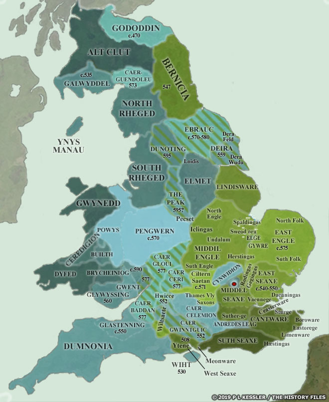
Map 4: AD 550-575
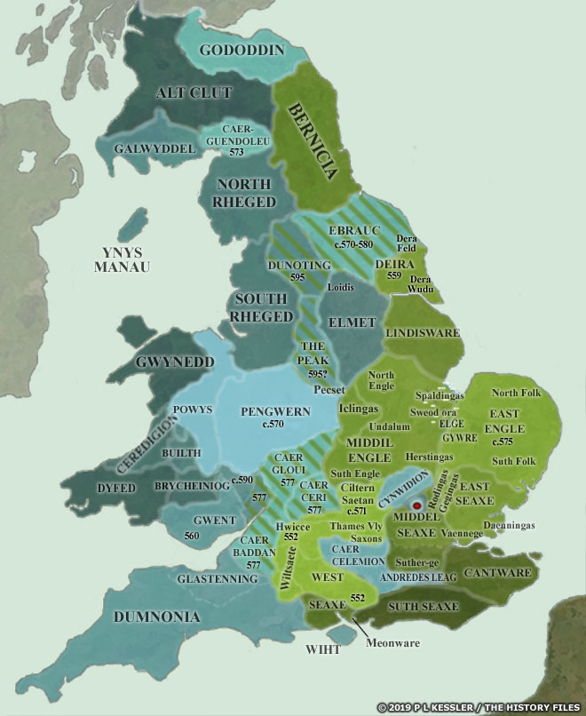
Map 5: AD 575-600
Map 6: AD 600-650
Map 7: AD 650-700
Map 8: AD 700
See: P.L. Kessler, Sequential Maps of the Anglo-Saxon Conquest AD 450-700, The History Files, 2023, https://www.historyfiles.co.uk/FeaturesBritain/BritishMapAD450-700.htm
[18] Gildas (c. 500–570 AD) was a sixth-century British monk, cleric, and historian known as Gildas Sapiens (“the Wise”). He is famous for writing De Excidio et Conquestu Britanniae, a sermon and historical account lamenting the decay of Britain and the destruction caused by the Saxon invasion.
Gildas, Wikipedia, This page was last edited on 24 February 2026, https://en.wikipedia.org/wiki/Gildas
Howells, Caleb, , Who Was Gildas? A Voice from Dark Age Britain, 17 Jul 2023, The Collector, https://www.thecollector.com/who-was-gildas/
[19] Limmer, Michael Sean, The Transformation of Identity in Early Medieval England: Continuity, Disruption, and Creolization, MA Thesis, University of New Mexico, Jul 2021, https://digitalrepository.unm.edu/cgi/viewcontent.cgi?article=1299&context=hist_etds
History of Anglo-Saxon England, Wikipedia, This page was last edited on 8 March 2026, https://en.wikipedia.org/wiki/History_of_Anglo-Saxon_England
Harland, James M., Rethinking Ethnicity and ›Otherness‹ in Early Anglo-Saxon England, medieval worlds, No. 5 , 2017, 113-142, https://medievalworlds.net/0xc1aa5572%200x00369e4f.pdf
Geary, Patrick J. , Ethnic identity as a situational construct in the early middle ages*), Mitteilungen der Anthropologischen Gesellschaft in Wien (MAGW) Band 113, 1983, S. 15-26, https://albert.ias.edu/server/api/core/bitstreams/7e261ae1-cfbd-4535-991d-1967cd4badf8/content
[20] Harland, James M., Rethinking Ethnicity and ›Otherness‹ in Early Anglo-Saxon England, medieval worlds, No. 5 , 2017, 113-142, https://medievalworlds.net/0xc1aa5572%200x00369e4f.pdf
History of Anglo-Saxon England, Wikipedia, This page was last edited on 8 March 2026, https://en.wikipedia.org/wiki/History_of_Anglo-Saxon_England
Limmer, Michael Sean, The Transformation of Identity in Early Medieval England: Continuity, Disruption, and Creolization, MA Thesis, University of New Mexico, Jul 2021, https://digitalrepository.unm.edu/cgi/viewcontent.cgi?article=1299&context=hist_etds
Roller, Sarah, The 4 Kingdoms that Dominated Early Medieval England, 15 October 2018, HistoryHit, https://www.historyhit.com/the-4-kingdoms-that-dominated-early-medieval-england/
Heptarchy, Wikipedia, This page was last edited on 8 January 2026, https://en.wikipedia.org/wiki/Heptarchy
Geary, Patrick J. , Ethnic identity as a situational construct in the early middle ages*), Mitteilungen der Anthropologischen Gesellschaft in Wien (MAGW) Band 113, 1983, S. 15-26, https://albert.ias.edu/server/api/core/bitstreams/7e261ae1-cfbd-4535-991d-1967cd4badf8/content
[21] Heptarchy, Wikipedia, This page was last edited on 8 January 2026, https://en.wikipedia.org/wiki/Heptarchy
[22] Geary, Patrick J. , Ethnic identity as a situational construct in the early middle ages*), Mitteilungen der Anthropologischen Gesellschaft in Wien (MAGW) Band 113, 1983, S. 15-26, https://albert.ias.edu/server/api/core/bitstreams/7e261ae1-cfbd-4535-991d-1967cd4badf8/content
Limmer, Michael Sean, The Transformation of Identity in Early Medieval England: Continuity, Disruption, and Creolization, MA Thesis, University of New Mexico, Jul 2021, https://digitalrepository.unm.edu/cgi/viewcontent.cgi?article=1299&context=hist_etds
Harland, James M., Rethinking Ethnicity and ›Otherness‹ in Early Anglo-Saxon England, medieval worlds, No. 5 , 2017, 113-142, https://medievalworlds.net/0xc1aa5572%200x00369e4f.pdf
Roller, Sarah, The 4 Kingdoms that Dominated Early Medieval England, 15 October 2018, HistoryHit, https://www.historyhit.com/the-4-kingdoms-that-dominated-early-medieval-england/
Heptarchy, Wikipedia, This page was last edited on 8 January 2026, https://en.wikipedia.org/wiki/Heptarchy
History of Anglo-Saxon England, Wikipedia, This page was last edited on 8 March 2026, https://en.wikipedia.org/wiki/History_of_Anglo-Saxon_England
[23] Anglo-Saxon royal houses (Kent, Wessex, Mercia, Northumbria, East Anglia) traced their lineage to the Germanic god Woden to legitimize their rule, a practice persisting into Christian times. Pedigrees often place Woden nine generations before key 5th-century founders like Hengest, linking him to the royal lines through sons such as Bældæg, Wægdæg, or Wecta.
Rowsell, Tom, Woden and his Roles in Anglo-Saxon Royal Genealogy. https://www.academia.edu/17509298/Woden_and_his_Roles_in_Anglo_Saxon_Royal_Genealogy
Anglo-Saxon royal genealogies, Wikipedia, This page was last edited on 11 March 2026, https://en.wikipedia.org/wiki/Anglo-Saxon_royal_genealogies
[24] Heptarchy, Wikipedia, This page was last edited on 8 January 2026, https://en.wikipedia.org/wiki/Heptarchy
History of Anglo-Saxon England, Wikipedia, This page was last edited on 8 March 2026, https://en.wikipedia.org/wiki/History_of_Anglo-Saxon_England
Geary, Patrick J. , Ethnic identity as a situational construct in the early middle ages*), Mitteilungen der Anthropologischen Gesellschaft in Wien (MAGW) Band 113, 1983, S. 15-26, https://albert.ias.edu/server/api/core/bitstreams/7e261ae1-cfbd-4535-991d-1967cd4badf8/content
Limmer, Michael Sean, The Transformation of Identity in Early Medieval England: Continuity, Disruption, and Creolization, MA Thesis, University of New Mexico, Jul 2021, https://digitalrepository.unm.edu/cgi/viewcontent.cgi?article=1299&context=hist_etds
Harland, James M., Rethinking Ethnicity and ›Otherness‹ in Early Anglo-Saxon England, medieval worlds, No. 5 , 2017, 113-142, https://medievalworlds.net/0xc1aa5572%200x00369e4f.pdf
[25] Laeti, Wikipedia, This page was last edited on 18 January 2026, https://en.wikipedia.org/wiki/Laeti
Goldsworthy, Adrian, Roman Warfare, Smithsonian Books, 2005, Page 215
[26] Jim Griffis, The Ancestor of Haplogroup G-Z6748, the Terps, Transport Corridors and Landscape Archaeology – Part Eight , January 14, 2026, Griffis Family: Selected Stries from the Past , https://griffis.org/the-ancestor-of-haplogroup-g-z6748-the-terps-transport-corridors-and-landscape-archaeology-part-eight/
Jim Griffis, The Ancestors of Haplogroup G-Z6748: A Frisian or Frank – Part Nine, February 11, 2026, Griffis family: Selected Stories from the past, https://griffis.org/the-ancestors-of-haplogroup-g-z6748-a-frisian-or-frank-part-nine/
[27] Between 570 to 850 CE, the English Channel was primarily known by its Roman-derived Latin name, Oceanus Britannicus (or Mare Britannicus), meaning the “British Ocean” or “Sea of the Britons”. It was also referred to as the “Narrow Sea” and Oceanus Gallicus (Gaulish Ocean) in some contexts. Other, often localized, names included the “British Sea” or simply the “Narrow Sea”. Various sources also identify it with Breton, such as Mor Breizh (Sea of Brittany).
Between 550 and 800 CE, during the early Middle Ages (roughly the Merovingian and early Viking period), the North Sea did not have a single universally standardized name, but it was generally referred to by Latin scholars as Oceanus Germanicus (German Ocean) or Mare Frisia (Frisian Sea).
English Chanel, Wikipedia, This page was last edited on 14 January 2026, https://en.wikipedia.org/wiki/English_Channel
North Sea, Wikipeida, This page was last edited on 2 March 2026, https://en.wikipedia.org/wiki/North_Sea
[28] Finding two Most Recent Common Ancestors (MRCAs) associated with two different SNP mutations only one or two generations apart is unusual but increasingly observed with modern, high-resolution sequencing (like BigY-700), which can detect very young, private mutations. This scenario implies that two distinct, consecutive SNP mutations occurred within a very short timeframe in the same lineage.
Detecting Single Nucleotide Polymorphism (SNP) mutations that are only one or two generations apart is considered unusual in the context of standard population genetics, but it is not impossible.
Most SNPs used in genealogy and ancestry testing arose thousands of years ago and are shared by thousands or millions of people. A mutation that occurs in a parental gamete and appears in a child is termed a de novo mutation, which is a rare event.
Possible Explanations
Data Misinterpretation/Calibration Error: The estimated time to the MRCA (TMRCA) can be influenced by the calibration methods (e.g., relying on STRs or incorrect generational assumptions). The apparent closeness might be a result of a shorter than expected “stem” in a phylogenetic tree.
Rapid Successive Mutation Events (“Hotspots”): The most straightforward explanation is that the first SNP occurred in a person, and in the next generation or two, a second SNP occurred in their descendant. While SNPs are rare, certain areas of the genome are more prone to mutation than others.
Recombination of Proximal Mutations: If the two SNPs are close together on the same chromosome, they might appear as two separate events, but could actually be part of a single, larger, complex rearrangement or simultaneous double mutation.
Reversion or Recurring Mutation: It is possible that the “second” mutation is actually a reversion, where the DNA mutates back to its ancestral state, or a new, different mutation occurs at the same site, making it appear as if two distinct ancestors were responsible for two separate changes within a short time.
Non-Linear Molecular Clock (SNP Rate Variation): Molecular clocks are averages. Some lineages might experience faster-than-average mutation rates (hot branches), leading to more mutations (and therefore more apparent MRCAs) in a shorter calendar time than expected.
Extremely Low Individual Rate: The human germline mutation rate results in 45–60 new de novo mutations in every person’s genome, the odds of a specific, identifiable SNP changing in a direct, close relative (parent-child) are very low.
“Rare” vs. “Common” SNPs: A “SNP” (by definition) is usually found in less than one percent of the population, implying it is old. A mutation occurring in one generation is technically a “rare variant” or a “singleton” (unique to that individual).
Paternal Age Factor: The number of de novo mutations is strongly influenced by the age of the father at conception, increasing by about 2 mutations per year. Therefore, if a parent is very old, the likelihood of a new SNP appearing in the child increases, though it is still rare.
Exceptions (Known Cases): In rare cases, a new SNP can appear in a child (e.g., in a sperm or egg cell) and be inherited, as was the case with the mutation causing Hemophilia in Queen Victoria’s lineage.
Is This Unusual? It is a rare, but plausible occurrence representing a “fast-moving” lineage or a highly mutable genomic region.
- Historically: Yes, it was considered unusual. SNP mutations were thought to take hundreds or thousands of years to accumulate.
- Presently: It is less unusual now. With high-coverage sequencing, “private” or very young SNP mutations are being discovered, and cases with small numbers of mutations (1-3) separating individuals are common in genealogical datasets.
Casci, T. SNPs that come in threes. Nat Rev Genet 11, 8 (2010). https://doi.org/10.1038/nrg2725
Scientific Details: A Deeper Dive Into Age Estimates, 19 Sep 2022, FamilyTreeDNA Blog, https://blog.familytreedna.com/tmrca-age-estimates-scientific-details/#:~:text=How%20a%20Relaxed%20Clock%20Model,lengths%2C%20and%20average%20the%20two.
Estes, Roberta, STRs vs SNPs, Multiple DNA Personalities, 10 Feb 2014, DNAeXplained – Genetic Genealogy, https://dna-explained.com/2014/02/10/strs-vs-snps-multiple-dna-personalities/
Waxman, D. and Gavrilets, S. (2005), 20 Questions on Adaptive Dynamics. Journal of Evolutionary Biology, 18: 1139-1154. https://doi.org/10.1111/j.1420-9101.2005.00948.x
Burbrink FT, Myers EA, Pyron RA. Understanding species limits through the formation of phylogeographic lineages. Ecol Evol. 2024 Oct 2;14(10):e70263. doi: 10.1002/ece3.70263. PMID: 39364037; PMCID: PMC11446989. https://pmc.ncbi.nlm.nih.gov/articles/PMC11446989/
Mohiuddin M, Kooy RF, Pearson CE. De novo mutations, genetic mosaicism and human disease. Front Genet. 2022 Sep 26;13:983668. doi: 10.3389/fgene.2022.983668. PMID: 36226191; PMCID: PMC9550265. https://pmc.ncbi.nlm.nih.gov/articles/PMC9550265/
Choudhury A, Hazelhurst S, Meintjes A, Achinike-Oduaran O, Aron S, Gamieldien J, Jalali Sefid Dashti M, Mulder N, Tiffin N, Ramsay M. Population-specific common SNPs reflect demographic histories and highlight regions of genomic plasticity with functional relevance. BMC Genomics. 2014 Jun 6;15(1):437. doi: 10.1186/1471-2164-15-437. PMID: 24906912; PMCID: PMC4092225. https://pmc.ncbi.nlm.nih.gov/articles/PMC4092225/
Haemophilia in European royalty, Wikipedia, This page was last edited on 17 November 2025, https://en.wikipedia.org/wiki/Haemophilia_in_European_royalty
[29] Cole, Lauren, Medieval myth busting: life expectancy, 10 Dec 2020, Medieval Lauren, https://medievallauren.wordpress.com/2020/12/10/medieval-myth-busting-life-expectancy/
David Musgrove, “Was the early medieval period a ‘golden age’ for the elderly?”, History Extra: https://www.historyextra.com/period/early-medieval/how-long-did-medieval-people-live-old-age-history/
Thijs Porck, “Old age as a prefiguration of Hell: Senescence in early medieval England”: https://thijsporck.com/2019/02/15/old-age/
M. A. Jonker, “Estimation of Life Expectancy in the Middle Ages”, Journal of the Royal Statistical Society, Vol. 166, No. 1 (2003), pp. 105-117
Thijs Porck, Old Age in Early Medieval England: A Cultural History (2019)
S. Shahar, “Who were old in the Middle Ages?”, Social History of Medicine (1993), pp.313-41
[30] Phylogeography, Wikipedia, This page was last edited on 3 October 2025, https://en.wikipedia.org/wiki/Phylogeography
Phylogeography, International Society of Genetic Genalogy Wiki, This page was last edited on 29 July 2021, https://isogg.org/wiki/Phylogeography
Avise, John C., The history and purview of phylogeography: a personal reflection, Molecular Ecology (1998) 7, 371–379, https://escholarship.org/content/qt1hv4f8vk/qt1hv4f8vk.pdf
[31] Estes, Roberta, Globetrekker – A New Feature for Big Y Customers From FamilyTreeDNA, 4 Aug 2023, DNAeXplained-Genetic Genealogy, https://dna-explained.com/2023/08/04/globetrekker-a-new-feature-for-big-y-customers-from-familytreedna/
Runfeldt, Goran, Globetrekker, Part 1: A New FamilyTreeDNA Discover™ Report That Puts Big Y on the Map, 31, Jul 2023, FamilyTreeDNA Blog, https://blog.familytreedna.com/globetrekker-discover-report
[32] See Jim Griffis, The Ancestors of Haplogroup G-Z6748: A Frisian or Frank – Part Nine, February 11, 2026, Griffis Family: Selected Stories from the Past, https://griffis.org/the-ancestors-of-haplogroup-g-z6748-a-frisian-or-frank-part-nine/
[33] English Chanel, Wikipedia, This page was last edited on 14 January 2026, https://en.wikipedia.org/wiki/English_Channel
[34] Maier, Paul, Part 2: Advancing the Science of Phylogeography, 15 Aug 2023, FamilyTreeDNA Blog, https://blog.familytreedna.com/globetrekker-analysis/
[35] Runfeldt, Goran, Globetrekker, Part 1: A New FamilyTreeDNA Discover™ Report That Puts Big Y on the Map, 31, Jul 2023, FamilyTreeDNA Blog, https://blog.familytreedna.com/globetrekker-discover-report/
Maier, Paul, Part 2: Advancing the Science of Phylogeography, 15 Aug 2023, FamilyTreeDNA Blog, https://blog.familytreedna.com/globetrekker-analysis/
[36] Maier, Paul, Part 2: Advancing the Science of Phylogeography, 15 Aug 2023, FamilyTreeDNA Blog, https://blog.familytreedna.com/globetrekker-analysis/
[37] Sub-Roman Britain, Wikipedia, This page was last edited on 16 February 2026,, https://en.wikipedia.org/wiki/Sub-Roman_Britain
Names of the British Isles, Wikipedia, This page was last edited on 13 February 2026, https://en.wikipedia.org/wiki/Names_of_the_British_Isles
British Isles, Wikipedia, This page was last edited on 8 February 2026, https://en.wikipedia.org/wiki/British_Isles
[38] See for example:
Gretzinger, J., Sayer, D., Justeau, P. et al. Author Correction: The Anglo-Saxon migration and the formation of the early English gene pool. Nature 611, E3 (2022). https://doi.org/10.1038/s41586-022-05429-y ; https://www.nature.com/articles/s41586-022-05247-2
Genetic and archaeological study reveals secrets of Medieval migration into England, 23 Sep 2022, Press Release PR-CDS-22-75, Cranfield University, https://www.cranfield.ac.uk/press/news-2022/the-anglo-saxon-migration-new-insights-from-genetics
Sedgeford featured in major ancient DNA publication, Sedgeford Historical and Archaeological Research Project (SHARP) Blog, https://www.sharp.org.uk/single-post/sedgeford-featured-in-major-ancient-dna-publication
Hills, C. M. “Did the people of Spong Hill come from Schleswig-Holstein.” Studien zur Sachsenforschung 11 (1999): 145-154.
“Spong Hill .” Ancient Europe, 8000 B.C. to A.D. 1000: Encyclopedia of the Barbarian World. Encyclopedia.com. 3 Feb. 2026, https://www.encyclopedia.com/humanities/encyclopedias-almanacs-transcripts-and-maps/spong-hill
Hills, Catherine M, “From Isidore to Isotopes: Ivory Rings in Early Medieval Graves.” In Image and Power in the Archaeology of Early Medieval Britain: Essays in Honour of Rosemary Cramp. Edited by Helena Hamerow and Arthur MacGregor, pp. 131–146. Oxford: Oxbow Books, 2001
Hills, Catherine M. Origins of the English. London: Duckworth, 2003
Hills, Catherine M., Kenneth J. Penn, and Robert J. Rickett. The Anglo-Saxon Cemetery at Spong Hill, North Elmham, Norfolk, Part V. East Anglian Archaeology, report no. 67. Norfolk, U.K.: Gressenhall, 1994.
McKinley, Jacqueline, The Anglo-Saxon cemetery at Spong Hill, North Elmham, Dereham, Norfolk : Norfolk Archaeological Unit, Norfolk Museums Service, https://archive.org/details/anglosaxoncemete0000unse/mode/2up
Anglo-Frisian Origins: Shared Heritage Across the North Sea, 22 May 2025, Ealdlar, https://ealdlar.com/history/anglo-frisian-origins
Anglo-Frisian History & Culture, Ealdlar, https://ealdlar.com/history
Migration Period Longboats: Seafaring and Inland Vessels (4th – 9th Centuries), https://ealdlar.com/history/frisian-longships
Van de Noort, Robert, North Sea Archaeologies, Oxford University Press, 2011, Page 171, https://www.ancientportsantiques.com/wp-content/uploads/Documents/PLACES/UK-EUNorth/NorthSea-VandeNoort2011.pdf
Martin Carver and Chris Loveluck with Stuart Brookes, Robin Daniels, Gareth Davies, Christopher Ferguson, Helen Geake, David Griffiths, David Hinton, Edward Oakley and Imogen Tompsett, The Early Medieval: An Maritime Archaeological Research Agenda for England, 2026, https://researchframeworks.org/maritime/early-medieval-ad-400-to-1000/
Green, Helen, A Review of North Sea Archaeologies: A Maritime Biography, 10,000 BC to AD 1500 by Robert Van de Noort, The Killingrove Review, Issue 11, https://www.gla.ac.uk/media/Media_279244_smxx.pdf
[39] See for example:
Van de Noort, Robert, North Sea Archaeologies, Oxford University Press, 2011, Page 171, https://www.ancientportsantiques.com/wp-content/uploads/Documents/PLACES/UK-EUNorth/NorthSea-VandeNoort2011.pdf
Loveluck, Chris & Dries Tys, Coastal societies, exchange and identity along the Channel and southern North Sea shores of Europe, AD 600–1000, Journal of Maritime Archaeology (2006) 1:141, DOI 10.1007/s11457-006-9007-x, https://www.academia.edu/1847904/Coastal_societies_exchange_and_identity_along_the_Channel_and_southern_North_Sea_shores_of_Europe_ad_600_1000
Wilken D, Hadler H, Wunderlich T, Majchczack B, Schwardt M, Fediuk A, Fischer P, Willershäuser T, Klooß S, Vött A, Rabbel W. Lost in the North Sea-Geophysical and geoarchaeological prospection of the Rungholt medieval dyke system (North Frisia, Germany). PLoS One. 2022 Apr 4;17(4):e0265463. doi: 10.1371/journal.pone.0265463. PMID: 35377888; PMCID: PMC8979465. https://pmc.ncbi.nlm.nih.gov/articles/PMC8979465/
IJssennagger-van der Pluijm N. Structured by the Sea: Rethinking Maritime Connectivity of the Early-Medieval Frisians. In: Hines J, IJssennagger-van der Pluijm N, eds. Frisians of the Early Middle Ages. Studies in Historical Archaeoethnology. Boydell & Brewer; 2021:249-272, https://www.cambridge.org/core/books/abs/frisians-of-the-early-middle-ages/structured-by-the-sea-rethinking-maritime-connectivity-of-the-earlymedieval-frisians/329B51FF63FDD5F6B2994E78BA3C072B
Anglo-Frisian Origins: Shared Heritage Across the North Sea, 22 May 2025, Ealdlar, https://ealdlar.com/history/anglo-frisian-origins
Anglo-Frisian History & Culture, Ealdlar, https://ealdlar.com/history
Migration Period Longboats: Seafaring and Inland Vessels (4th – 9th Centuries), https://ealdlar.com/history/frisian-longships
Van de Noort, Robert, North Sea Archaeologies, Oxford University Press, 2011, Page 171, https://www.ancientportsantiques.com/wp-content/uploads/Documents/PLACES/UK-EUNorth/NorthSea-VandeNoort2011.pdf
Martin Carver and Chris Loveluck with Stuart Brookes, Robin Daniels, Gareth Davies, Christopher Ferguson, Helen Geake, David Griffiths, David Hinton, Edward Oakley and Imogen Tompsett, The Early Medieval: An Maritime Archaeological Rresearch Agenda for England, 2026, https://researchframeworks.org/maritime/early-medieval-ad-400-to-1000/
Green, Helen, A Review of North Sea Archaeologies: A Maritime Biography, 10,000 BC to AD 1500 by Robert Van de Noort, The Killingrove Review, Issue 11, https://www.gla.ac.uk/media/Media_279244_smxx.pdf
[40] Loveluck, Chris & Dries Tys, Coastal societies, exchange and identity along the Channel and southern North Sea shores of Europe, AD 600–1000, Journal of Maritime Archaeology (2006) 1:141, DOI 10.1007/s11457-006-9007-x, https://www.academia.edu/1847904/Coastal_societies_exchange_and_identity_along_the_Channel_and_southern_North_Sea_shores_of_Europe_ad_600_1000
[41] Wics or emporia were characterised by their peripheral locations, usually on the shore at the edge of a kingdom, their lack of infrastructure (containing no churches) and their short-lived nature. Typically, a wic (an Anglo-Saxon word) would have no church or high status residence, hinting that they were almost entirely oriented towards trade. This is emphasised by the way in wics were usually twinned with other settlements. By 1000 CE , the emporia had been replaced by the revival of European towns.
Early Medieval Emporia, Early Medieval Archaeology, http://early-med.archeurope.com/emporia/
Marissa, Which Wic?, 3 Jul 2012, Mediedal Musings, https://mediaevalmusings.wordpress.com/2012/07/03/which-wic/
Dalwood, Hal, ‘Water, Wics and Burhs’, in Maren Clegg Hyer, and Della Hooke (eds), Water and the Environment in the Anglo-Saxon World, Liverpool, 2018; online edn, Liverpool Scholarship Online, 24 May 2018), https://doi.org/10.5949/liverpool/9781786940285.003.0010,
Crabtree PJ. Middle Saxon Settlement and the Rise of the Emporia: The Archaeology of the Wics and Contemporary Sites. In: Early Medieval Britain: The Rebirth of Towns in the Post-Roman West. Case Studies in Early Societies. Cambridge University Press; 2018:86-137. https://www.cambridge.org/core/books/abs/early-medieval-britain/middle-saxon-settlement-and-the-rise-of-the-emporia-the-archaeology-of-the-wics-and-contemporary-sites/0800C45C886B344E30A2C9FB9AFD97AD
Michael Dietler, Eric Gailledrat, Rosa Plana-Mallart. The Emporion in Context. Michael Dietler; Eric Gailledrat; Rosa Plana-Mallart. The emporion in the Ancient Western Mediterranean. Trade and Colonial Encounters from the Archaic to the Hellenistic Period, Presses Universitaires de la Méditerranée, pp.11-16, 2018, Mondes Anciens, 978-2-36781-275-5. halshs-05229729, https://shs.hal.science/halshs-05229729/document
[42] See the following for a core set of “maritime” and “seascape” oriented works that focus on the North Sea and Dutch and English coasts during 500 – 800 CE:
North Sea–Wide Seascapes and Theoretical Models:
- Van de Noort, R. 2011. North Sea Archaeologies: A Maritime Biography, 10,000 BC–AD 1500. Oxford University Press. https://www.ancientportsantiques.com/wp-content/uploads/Documents/PLACES/UK-EUNorth/NorthSea-VandeNoort2011.pdf . Van de Noort develops an explicitly seascape and “maritime biography” based framework for the North Sea, with substantial discussion of the early medieval period and the Frisia–England axis.
- Hines, J., and N. IJssennagger (eds.). Frisians and their North Sea World: from Migration to the Middle Ages. Boydell & Brewer. 2017,
Several chapters of this collection of articles treat the North Sea as a connective maritime zone; note especially Hines on the “Anglo‑Frisian question”, IJssennagger on emporia and seafaring links and Pestell on English east coast and emporia as seascapes. https://www.cambridge.org/core/books/frisians-and-their-north-sea-neighbours/3E63327F4D3842542B0E1DD40129BE3B - See also Bev Thurber’s review: 18.09.20, Hines/IJssennagger (eds.), Frisians and their North Sea Neighbours, Medieval Review, https://scholarworks.iu.edu/journals/index.php/tmr/article/view/25647
- Chris Loveluck and Dries Tys, Coastal societies, exchange and identity along the Channel and southern North Sea shores of Europe, AD 600–1000, J Mari Arch (11 Nov 2006) 1:140–169, DOI 10.1007/s11457-006-9007-x , https://www.academia.edu/1847904/Coastal_societies_exchange_and_identity_along_the_Channel_and_southern_North_Sea_shores_of_Europe_ad_600_1000 Loveluck and Tys explore the functioning of coastal societies against the background of the changing role of coastal ‘contact zones’ on both sides of the Channel and southern North Sea region. Their article is a classic articulation of coastal communities and contact zones as socially constructed maritime landscapes rather than mere edges of terrestrial polities.
- Martin Carver and Chris Loveluck with Stuart Brookes, Robin Daniels, Gareth Davies, Christopher Ferguson, Helen Geake, David Griffiths, David Hinton, Edward Oakley and Imogen Tompsett, The Early Medieval: An Maritime Archaeological Rresearch Agenda for England, 2026, https://researchframeworks.org/maritime/early-medieval-ad-400-to-1000/ . These researchers provide a research agenda that explicitly frames the English early medieval coast as a dynamic seascape of land‑reclamation, estuarine exploitation, and maritime connectivity (Frisia–eastern England links are foregrounded).
Early medieval Frisia and Dutch coastal zone:
- Gilles de Langen, J. A. Mol “Landscape, Trade and Power in Early‑Medieval Frisia ” In Hines & IJssennagger, eds, Frisians of the Early Middle Ages, Boydell & Brewer; 2021. The authors use a spatial and landscape approach to question the coherence and the traditional “maritime” character of Frisia as a linear coastal strip (Bruges to Bremen). They reconstruct a regionally varied, predominantly rural society in which power and “Frisian” identity were unevenly structured and in important respects centered in West Frisia/Holland rather than the terp districts alone.
- Nelleke IJssennagger-van der Pluijm, “Structured by the Sea: Rethinking Maritime Connectivity of the Early-Medieval Frisians” In Hines & IJssennagger, Frisians of the Early Middle Ages. The author traces long‑term, cross‑North‑Sea links (trade, mobility, cultural exchange) and treats them as structural features of Frisian life rather than episodic contacts. By comparing Frisia with other coastal and seafaring cultures around the North Sea, she highlights shared coastal cultural zones and questions sharp political or ethnic boundaries in the maritime sphere.
- McManus, Ellen & Montgomery, Janet & Evans, Jane & Lamb, Angela & Brettell, Rhea & Jelsma, Johan. (2013), “To the Land or to the Sea”: Diet and Mobility in Early Medieval Frisia. The Journal of Island and Coastal Archaeology. 8. (2013) 255-277. 10.1080/15564894.2013.787565. See also: https://nora.nerc.ac.uk/id/eprint/504785/1/McManus%20et%20al%20-%20Oosterbeintum_final.pdf . The authors combine isotopes and archaeology to argue that Frisian coastal communities were strongly embedded in maritime trade and exploitation, treating sea/shore as an integrated economic and social environment.
- Deckers, Pieterjan & Dries Tys, Early medieval communities around the North Sea: a ‘maritime culture’?, in Rica Annaert, Tinne Jacobs, Ingrid In ’t Ven & Steffi Coppens, eds, ACE Conference of Brussels: The Very beginning of Europe? Early Medieval Migration and Colonization, 2012, 81-88, https://oar.onroerenderfgoed.be/publicaties/RELM/7/RELM007-001.pdf. The authors position Frisian coastal settlements and terpen within a network of maritime interactions; emphasizes the North Sea as a unifying medium for six6th–eighth century communities.
English east coast and emporia as seascapes:
- Martin Carver and Chris Loveluck with Stuart Brookes, Robin Daniels, Gareth Davies, Christopher Ferguson, Helen Geake, David Griffiths, David Hinton, Edward Oakley and Imogen Tompsett, The Early Medieval: An Maritime Archaeological Rresearch Agenda for England, 2026, https://researchframeworks.org/maritime/early-medieval-ad-400-to-1000/ . The English maritime research framework chapter cites Loveluck as key for understanding permanent occupation in low‑lying marshland and sand‑island sites from Humber to the Fens as coastal settlements embedded in tidal seascapes rather than marginal wetlands.
[43] Van de Noort, Robert, North Sea Archaeologies, Oxford University Press, 2011, Page 171, https://www.ancientportsantiques.com/wp-content/uploads/Documents/PLACES/UK-EUNorth/NorthSea-VandeNoort2011.pdf
For reviews of Vande Noort’s work, see:
Farr, R. H. (2011). [Review of North Sea Archaeologies: A Maritime Biography, 10,000 BC-AD 1500, by R. Van de Noort]. Journal of Maritime Archaeology, 6(1), 91–93. http://www.jstor.org/stable/43551364
Farr, Helen, Book review. Robert Van de Noort: North Sea Archaeologies: A Maritime Biography, 10,000 BC–AD 1500, July 2011, Journal of Maritime Archaeology 6(1), https://www.researchgate.net/publication/313311229_Book_review_Robert_Van_de_Noort_North_Sea_Archaeologies_A_Maritime_Biography_10000_BC-AD_1500
Fitch, Simon, North Sea Archaeologies: A Maritime Biography, 10,000 BC – AD 1500.
Robert Van de Noort, Northern Scotland, 22 April 2013 Volume 4, Issue 1, https://doi.org/10.3366/nor.2013.00
Green, Helen, North Sea Archaeologies: A Maritime Biography, 10,000 BC to AD 1500, The Kelvingrove Review, Issue 11, https://www.gla.ac.uk/media/Media_279244_smxx.pdf
[44] Ealdlar, Anglo-Frisian Origins: Shared Heritage Across the North Sea, 22 May 2025, Ealdlar, https://ealdlar.com/history/anglo-frisian-origins
[45] Van de Noort, Robert, North Sea Archaeologies, Oxford University Press, 2011, https://www.ancientportsantiques.com/wp-content/uploads/Documents/PLACES/UK-EUNorth/NorthSea-VandeNoort2011.pdf
Martin Carver and Chris Loveluck with Stuart Brookes, Robin Daniels, Gareth Davies, Christopher Ferguson, Helen Geake, David Griffiths, David Hinton, Edward Oakley and Imogen Tompsett, The Early medieval, https://researchframeworks.org/maritime/early-medieval-ad-400-to-1000/
Ellen McManus, Janet Montgomery, Jane Evans , Angela Lamb, Rhea Brettell, Johan Jelsma, ‘To the land or to the sea’: diet and mobility in early medieval Frisia, https://nora.nerc.ac.uk/id/eprint/504785/1/McManus%20et%20al%20-%20Oosterbeintum_final.pdf
Deckers, Pieterjan & Dries Tys, Early medieval communities around the North Sea: a ‘maritime culture’?, in Rica Annaert, Tinne Jacobs, Ingrid In ’t Ven & Steffi Coppens, eds, ACE Conference of Brussels: The Very beginning of Europe? Early Medieval Migration and Colonization, 2012, 81-88, https://oar.onroerenderfgoed.be/publicaties/RELM/7/RELM007-001.pdf
Migration Period Longboats: Seafaring and Inland Vessels (4th-9th Centuries), Ealdlar, https://ealdlar.com/history/frisian-longships
Bruce-Mitford, Rupert Leo Scott, The Sutton Hoo ship-burial, London : British Museum Publications Ltd. 1975, https://archive.org/details/suttonhooshipbur0000bruc/page/n1/mode/2up
Greenhill, B. The Archaeology of Boats & Ships: An Introduction. Conway Maritime Press 1995,
McGrail, Seán, Ancient Boats in North-West Europe The archaeology of water transport to AD 1500, New York: Routledge, 1988 , https://dokumen.pub/qdownload/ancient-boats-in-north-west-europe-the-archaeology-of-water-transport-to-ad-1500-revised-058249267x-9780582492677.html
Knol E, Ijssennagger N. Palaeogeography and People: Historical Frisians in an archaeological light. In: Hines J, IJssennagger N, eds. Frisians and Their North Sea Neighbours: From the Fifth Century to the Viking Age. Boydell & Brewer; 2017:5-24,
[46] Loveluck, Chris & Dries Tys, Coastal societies, exchange and identity along the Channel and southern North Sea shores of Europe, AD 600–1000, Journal of Maritime Archaeology (2006) 1:141, DOI 10.1007/s11457-006-9007-x, https://www.academia.edu/1847904/Coastal_societies_exchange_and_identity_along_the_Channel_and_southern_North_Sea_shores_of_Europe_ad_600_1000
Wilken D, Hadler H, Wunderlich T, Majchczack B, Schwardt M, Fediuk A, Fischer P, Willershäuser T, Klooß S, Vött A, Rabbel W. Lost in the North Sea-Geophysical and geoarchaeological prospection of the Rungholt medieval dyke system (North Frisia, Germany). PLoS One. 2022 Apr 4;17(4):e0265463. doi: 10.1371/journal.pone.0265463. PMID: 35377888; PMCID: PMC8979465. https://pmc.ncbi.nlm.nih.gov/articles/PMC8979465/
IJssennagger-van der Pluijm N. Structured by the Sea: Rethinking Maritime Connectivity of the Early-Medieval Frisians. In: Hines J, IJssennagger-van der Pluijm N, eds. Frisians of the Early Middle Ages. Studies in Historical Archaeoethnology. Boydell & Brewer; 2021:249-272, https://www.cambridge.org/core/books/abs/frisians-of-the-early-middle-ages/structured-by-the-sea-rethinking-maritime-connectivity-of-the-earlymedieval-frisians/329B51FF63FDD5F6B2994E78BA3C072B
Anglo-Frisian Origins: Shared Heritage Across the North Sea, 22 May 2025, Ealdlar, https://ealdlar.com/history/anglo-frisian-origins
Anglo-Frisian History & Culture, Ealdlar, https://ealdlar.com/history
Kemp, John and Brian D’Olier, Early Navigation in the North Sea – The Use of the Lead and Line and other Navigation Methods, The Journal of Navigation (2016), 69, 673–697. © The Royal Institute of Navigation 2015 doi:10.1017/S0373463315000934, https://www.academia.edu/90523151/Early_Navigation_in_the_North_Sea_The_Use_of_the_Lead_and_Line_and_other_Navigation_Methods
Kemp, John, The Use of the Lead and Line by Early Navigators in the North Sea?, TransNav, Volume 8 Number 4 Dec 2014, DOI 10.12716/1001.08.04.01, 481 – 483
[47] Migration Period Longboats: Seafaring and Inland Vessels (4th-9th Centuries), Ealdlar, https://ealdlar.com/history/frisian-longships
[48] Migration Period Longboats: Seafaring and Inland Vessels (4th-9th Centuries), Ealdlar,https://ealdlar.com/history/frisian-longships
[49] Van de Noort, Robert, North Sea Archaeologies, Oxford University Press, 2011, Page 171, https://www.ancientportsantiques.com/wp-content/uploads/Documents/PLACES/UK-EUNorth/NorthSea-VandeNoort2011.pdf
[50] The Humber–southern Jutland corridor is a geomorphological and maritime band across the southern North Sea: from the Humber estuary on England’s east coast to the south‑west coast of Jutland (via Schleswig/Funen), marking the southern “inner sea” zone where Holocene subsidence and sea‑level rise drowned a former lowland into today’s shallow North Sea.
In seascape archaeology, that line effectively separates a shallow, bank‑filled “inner North Sea” from deeper northern basins, creating a corridor of relatively predictable tides and short‑haul crossings between estuaries and barrier‑island coasts. Early medieval maritime research treats the Humber estuary and adjacent coast (Humber–Fens) on the west, and the Wadden/Jutland coast on the east, as a coherent coastal system of landing places, beach markets and emporia rather than isolated shores.
Van de Noort, Robert, North Sea Archaeologies, Oxford University Press, 2011, https://www.ancientportsantiques.com/wp-content/uploads/Documents/PLACES/UK-EUNorth/NorthSea-VandeNoort2011.pdf
Westerdahl, Christer, The Maritime Cultural Landscape: On the concept of the traditional zones of transport geography, 1998, Inst of Archaeology and Ethnology, University of Copenhagen, https://www.abc.se/~pa/publ/cult-land.htm
Loveluck C. Ports and maritime-oriented societies, AD 600–900. In: Northwest Europe in the Early Middle Ages, c.AD 600–1150: A Comparative Archaeology. Cambridge University Press; 2013:178-212. https://www.cambridge.org/core/books/abs/northwest-europe-in-the-early-middle-ages-cad-6001150/ports-and-maritimeoriented-societies-ad-600900/6DF0F99C5490E9592CBC879E9457A4C7
Van de Noort, Robert, Argonauts of the North Sea: Social Maritime Archaeology, 2nd Milleium BC,, 2006, Proceedings of the Prehistoric Society, pp. 267–287, https://www.academia.edu/3663229/Argonauts_of_the_North_Sea
Bente Sven Majchczack, A new light on early medieval North Frisia: Harbours and trading sites on the islands of Föhr and Sylt, Pages 161 – 184, in Babette Ludowici and Heike Pöppelmann, eds, New Narratives for the First Millennium AD?, Braunschweigisches Landesmuseum Alle Rechte vorbehalten , 2022, https://www.academia.edu/127066328/A_new_light_on_early_medieval_North_Frisia_Harbours_and_trading_sites_on_the_islands_of_Föhr_and_Sylt
Hines J, IJssennagger N, eds. Frisians and Their North Sea Neighbours: From the Fifth Century to the Viking Age. Boydell & Brewer; 2017. https://www.cambridge.org/core/books/frisians-and-their-north-sea-neighbours/3E63327F4D3842542B0E1DD40129BE3B
Hines J, Ijssennagger N. Introduction: Frisians – Who, When, Where, Why? In: Hines J, IJssennagger N, eds. Frisians and Their North Sea Neighbours: From the Fifth Century to the Viking Age. Boydell & Brewer; 2017:1-4.
Hines J. The Anglo-Frisian Question. In: Hines J, IJssennagger N, eds. Frisians and Their North Sea Neighbours: From the Fifth Century to the Viking Age. Boydell & Brewer; 2017:25-42.
Dijkstra M, Koning J de. ‘All quiet on the Western Front?’ The Western Netherlands and the ‘North Sea Culture’ in the Migration Period. In: Hines J, IJssennagger N, eds. Frisians and Their North Sea Neighbours: From the Fifth Century to the Viking Age. Boydell & Brewer; 2017:53-74.
Pestell T. The Kingdom of East Anglia, Frisia and Continental Connections, c. ad 600–900. In: Hines J, IJssennagger N, eds. Frisians and Their North Sea Neighbours: From the Fifth Century to the Viking Age. Boydell & Brewer; 2017:193-222.
[51] Loveluck C. Ports and maritime-oriented societies, AD 600–900. In: Northwest Europe in the Early Middle Ages, c.AD 600–1150: A Comparative Archaeology. Cambridge University Press; 2013:178-212. https://www.cambridge.org/core/books/abs/northwest-europe-in-the-early-middle-ages-cad-6001150/ports-and-maritimeoriented-societies-ad-600900/6DF0F99C5490E9592CBC879E9457A4C7
Martin Carver and Chris Loveluck with Stuart Brookes, Robin Daniels, Gareth Davies, Christopher Ferguson, Helen Geake, David Griffiths, David Hinton, Edward Oakley and Imogen Tompsett, The Early Medieval: An Maritime Archaeological Research Agenda for England, 2026, https://researchframeworks.org/maritime/early-medieval-ad-400-to-1000/
Pestell T. The Kingdom of East Anglia, Frisia and Continental Connections, c. ad 600–900. In: Hines J, IJssennagger N, eds. Frisians and Their North Sea Neighbours: From the Fifth Century to the Viking Age. Boydell & Brewer; 2017:193-222.
[52] Knol E, Ijssennagger N. Palaeogeography and People: Historical Frisians in an archaeological light. In: Hines J, IJssennagger N, eds. Frisians and Their North Sea Neighbours: From the Fifth Century to the Viking Age. Boydell & Brewer; 2017:5-24. https://www.cambridge.org/core/books/abs/frisians-and-their-north-sea-neighbours/palaeogeography-and-people-historical-frisians-in-an-archaeological-light/CA5BEE0DAC45640D30C3E40FBDC11C49
Martin Carver and Chris Loveluck with Stuart Brookes, Robin Daniels, Gareth Davies, Christopher Ferguson, Helen Geake, David Griffiths, David Hinton, Edward Oakley and Imogen Tompsett, The Early Medieval: An Maritime Archaeological Research Agenda for England, 2026, https://researchframeworks.org/maritime/early-medieval-ad-400-to-1000/
Van de Noort, Robert, North Sea Archaeologies, Oxford University Press, 2011, https://www.ancientportsantiques.com/wp-content/uploads/Documents/PLACES/UK-EUNorth/NorthSea-VandeNoort2011.pdf
Hines J. The Anglo-Frisian Question. In: Hines J, IJssennagger N, eds. Frisians and Their North Sea Neighbours: From the Fifth Century to the Viking Age. Boydell & Brewer; 2017:25-42.
[53] Chris Loveluck and Dries Tys, Coastal societies, exchange and identity along the Channel and southern North Sea shores of Europe, AD 600–1000, J Mari Arch (11 Nov 2006) 1:140–169, DOI 10.1007/s11457-006-9007-x , https://www.academia.edu/1847904/Coastal_societies_exchange_and_identity_along_the_Channel_and_southern_North_Sea_shores_of_Europe_ad_600_1000
Knol E, Ijssennagger N. Palaeogeography and People: Historical Frisians in an archaeological light. In: Hines J, IJssennagger N, eds. Frisians and Their North Sea Neighbours: From the Fifth Century to the Viking Age. Boydell & Brewer; 2017:5-24. https://www.cambridge.org/core/books/abs/frisians-and-their-north-sea-neighbours/palaeogeography-and-people-historical-frisians-in-an-archaeological-light/CA5BEE0DAC45640D30C3E40FBDC11C49
Martin Carver and Chris Loveluck with Stuart Brookes, Robin Daniels, Gareth Davies, Christopher Ferguson, Helen Geake, David Griffiths, David Hinton, Edward Oakley and Imogen Tompsett, The Early Medieval: An Maritime Archaeological Research Agenda for England, 2026, https://researchframeworks.org/maritime/early-medieval-ad-400-to-1000/
Van de Noort, Robert, North Sea Archaeologies, Oxford University Press, 2011, https://www.ancientportsantiques.com/wp-content/uploads/Documents/PLACES/UK-EUNorth/NorthSea-VandeNoort2011.pdf
[54] Chris Loveluck and Dries Tys, Coastal societies, exchange and identity along the Channel and southern North Sea shores of Europe, AD 600–1000, J Mari Arch (11 Nov 2006) 1:140–169, DOI 10.1007/s11457-006-9007-x , https://www.academia.edu/1847904/Coastal_societies_exchange_and_identity_along_the_Channel_and_southern_North_Sea_shores_of_Europe_ad_600_1000
[55] Chris Loveluck and Dries Tys, Coastal societies, exchange and identity along the Channel and southern North Sea shores of Europe, AD 600–1000, J Mari Arch (11 Nov 2006) 1:140–169, DOI 10.1007/s11457-006-9007-x , https://www.academia.edu/1847904/Coastal_societies_exchange_and_identity_along_the_Channel_and_southern_North_Sea_shores_of_Europe_ad_600_1000
[56] Chris Loveluck and Dries Tys, Coastal societies, exchange and identity along the Channel and southern North Sea shores of Europe, AD 600–1000, J Mari Arch (11 Nov 2006) 1:140–169, DOI 10.1007/s11457-006-9007-x , https://www.academia.edu/1847904/Coastal_societies_exchange_and_identity_along_the_Channel_and_southern_North_Sea_shores_of_Europe_ad_600_1000
[57] Tys, Dries, Maritime and River Traders, Landing Places, and Emporia Ports in the Merovingian Period in and Around the Low Countries, 1 – 36 printed from Oxford Handbooks online (www.oxfordhandbooks.com). Oxford University Press, 2018. Online Publication Date: Oct 2020, DOI: 10.1093/oxfordhb/9780190234188.013.26, https://www.academia.edu/93991995/Maritime_and_River_Traders_Landing_Places_and_Emporia_Ports_in_the_Merovingian_Period_in_and_Around_the_Low_Countries
Sindbæk, Søren M. , Emporia, high-definition archaeology, and Ribe, 11- 23, in Northern Emporium, Sindbæk, Søren M., editor. Northern Emporium: Vol. 1 The Making of Viking-Age Ribe. vol. 122, Aarhus University Press, 2022. JSTOR, https://doi.org/10.2307/j.ctv33jb4rt.
Hines J, IJssennagger N, eds. Frisians and Their North Sea Neighbours: From the Fifth Century to the Viking Age. Boydell & Brewer; 2017. https://www.cambridge.org/core/books/frisians-and-their-north-sea-neighbours/3E63327F4D3842542B0E1DD40129BE3B
Early Medieval Trade between Anglo-Saxon England and Frisia, Ealdlar, https://ealdlar.com/early-medieval-trade
[58] Archaeological evidence from the fifth century points to significant early Germanic settlement in England, with Spong Hill in Norfolk and Mucking in Essex serving as key examples of this transition. These sites provide crucial evidence of the migration, culture, and daily life of the incoming Anglo-Saxons. The cemeteries contain distinctive Germanic-style, urn-field cremations (similar to those in northern Germany) and, in some cases, furnished inhumations with grave goods.
Key Archaeological Evidence:
Mucking, Essex: This site represents one of the most extensive Anglo-Saxon settlements excavated in Britain, featuring over 200 Grubenhauser (sunken huts), dozens of timber halls, and two cemeteries. Located on the Thames Estuary, Mucking shows early Germanic activity starting in the early 5th century.
Spong Hill, Norfolk: Known as the largest early Anglo-Saxon cremation cemetery in Britain, excavations at Spong Hill revealed over 2,200 cremation burials and 57 inhumations, along with associated sunken-featured buildings (Grubenhauser). The findings show the site was in use for roughly 150 years, starting in the early 5th century, and suggests the presence of Germanic settlers may predate traditional accounts (AD 450).
See also:
Faber, Hans, Merciless Medieval Merchants and Slavers, 19 Jun 2020, Frisia Coast Trail, https://www.frisiacoasttrail.com/post/merciless-medieval-merchants
Faber, Hans, The Batwing Doors of Dorestad. A Two-Way Gateway of Trade and Power, 13 April, 2020, Salt, Samphire & Storytellers, Friasian Coast Trail, https://www.frisiacoasttrail.com/post/2020/04/13/the-batwing-doors-of-northwest-europe
Bentonian, Dorestad, crossroads of the north, 30 Jun 2017, The Eighth Century and All of That, https://www.8thcentury.com/dorestad-crossroads-of-the-north/
Ealdlar, Early Medieval Trade between Anglo-Saxon England and Frisia, Ealdlar, https://ealdlar.com/early-medieval-trade
Kosian, Menne and Henk Weerts, Rowin Van Lanen, Jaap Evert Abrahamse, The City and the River. The early medieval Emporium (trade centre) of Dorestad; integrating physical geography with archaeological data in changing environments, International Conference on Cultural Heritage and New Technologies, Vienna, 2012, https://www.academia.edu/5851685/The_City_and_the_River_The_early_medieval_Emporium_trade_centre_of_Dorestad_integrating_physical_geography_with_archaeological_data_in_changing_environments
[59] Anglo-Frisian History & Culture, Ealdlar, https://ealdlar.com/history
[60] Chris Loveluck and Dries Tys, Coastal societies, exchange and identity along the Channel and southern North Sea shores of Europe, AD 600–1000, J Mari Arch (11 Nov 2006) 1:140–169, DOI 10.1007/s11457-006-9007-x , https://www.academia.edu/1847904/Coastal_societies_exchange_and_identity_along_the_Channel_and_southern_North_Sea_shores_of_Europe_ad_600_1000
Chris Loveluck and Dries Tys, Coastal societies, exchange and identity along the Channel and southern North Sea shores of Europe, AD 600–1000, J Mari Arch (11 Nov 2006) 1:140–169, DOI 10.1007/s11457-006-9007-x , https://www.academia.edu/1847904/Coastal_societies_exchange_and_identity_along_the_Channel_and_southern_North_Sea_shores_of_Europe_ad_600_1000
Deckers P. Cultural Convergence in a Maritime Context: Language and material culture as parallel phenomena in the early-medieval southern North Sea region. In: Hines J, IJssennagger N, eds. Frisians and Their North Sea Neighbours: From the Fifth Century to the Viking Age. Boydell & Brewer; 2017:173-192 , https://www.cambridge.org/core/books/abs/frisians-and-their-north-sea-neighbours/cultural-convergence-in-a-maritime-context-language-and-material-culture-as-parallel-phenomena-in-the-earlymedieval-southern-north-sea-region/05DD2C1DBDC0C6A6DB11D337D2CBB32A
Knol E, Ijssennagger N. Palaeogeography and People: Historical Frisians in an archaeological light. In: Hines J, IJssennagger N, eds. Frisians and Their North Sea Neighbours: From the Fifth Century to the Viking Age. Boydell & Brewer; 2017:5-24., https://www.cambridge.org/core/books/abs/frisians-and-their-north-sea-neighbours/palaeogeography-and-people-historical-frisians-in-an-archaeological-light/CA5BEE0DAC45640D30C3E40FBDC11C49
Van de Noort, Robert, North Sea Archaeologies, Oxford University Press, 2011, Page 171, https://www.ancientportsantiques.com/wp-content/uploads/Documents/PLACES/UK-EUNorth/NorthSea-VandeNoort2011.pdf
Early Medieval Trade between Anglo-Saxon England and Frisia, Ealdlar, https://ealdlar.com/early-medieval-trade
Anglo-Frisian History & Culture, Ealdlar, https://ealdlar.com/history
Research publications, Fryske Akademy,page Accessed 3 Mar 2026, https://www.fryske-akademy.nl/en/research/research-publications/
Majchczack, Bente Sven, A new light on early medieval North Frisia: Harbours and trading sites on the islands of Föhr and Sylt, in Babette Ludowici and Heike Pöppelmann, eds, New Narratives for the First Millennium AD?, Braunschweigisches Landesmuseum, 2022, https://www.academia.edu/127066328/A_new_light_on_early_medieval_North_Frisia_Harbours_and_trading_sites_on_the_islands_of_Föhr_and_Sylt
Lebecq, Stéphane The Frisian trade in the Dark Ages; a Frisian or a Frankish/Frisian trade? In: Carmiggelt, A.,(ed). Rotterdam Papers VII, 1992, pp. 7-15, https://www.scribd.com/doc/6919218/Lebecq-The-Frisian-trade-in-the-Dark-Ages
Sedgeford featured in major ancient DNA publication, Sedgeford Historical and Archaeological Research Project (SHARP) Blog, https://www.sharp.org.uk/single-post/sedgeford-featured-in-major-ancient-dna-publication
Hills, C. M. “Did the people of Spong Hill come from Schleswig-Holstein.” Studien zur Sachsenforschung 11 (1999): 145-154.
“Spong Hill .” Ancient Europe, 8000 B.C. to A.D. 1000: Encyclopedia of the Barbarian World. Encyclopedia.com. 3 Feb. 2026, https://www.encyclopedia.com/humanities/encyclopedias-almanacs-transcripts-and-maps/spong-hill
Hills, Catherine M, “From Isidore to Isotopes: Ivory Rings in Early Medieval Graves.” In Image and Power in the Archaeology of Early Medieval Britain: Essays in Honour of Rosemary Cramp. Edited by Helena Hamerow and Arthur MacGregor, pp. 131–146. Oxford: Oxbow Books, 2001
Hills, Catherine M. Origins of the English. London: Duckworth, 2003
Hills, Catherine M., Kenneth J. Penn, and Robert J. Rickett. The Anglo-Saxon Cemetery at Spong Hill, North Elmham, Norfolk, Part V. East Anglian Archaeology, report no. 67. Norfolk, U.K.: Gressenhall, 1994.
McKinley, Jacqueline, The Anglo-Saxon cemetery at Spong Hill, North Elmham, Dereham, Norfolk : Norfolk Archaeological Unit, Norfolk Museums Service, https://archive.org/details/anglosaxoncemete0000unse/mode/2up
[61] Faber, Hans, The Batwing Doors of Dorestad. A Two-Way Gateway of Trade and Power, 26 Oct, 2020, Frisian Coast Trail, https://frisiacoasttrail.blog/2020/10/26/dorestat/
Dorstad, Wikipedia, This page was last edited on 16 December 2024, https://en.wikipedia.org/wiki/Dorestad
W.A. van Es & W.J.H. Verwers, Early Medieval settlements along the Rhine: precursors and contemporaries of Dorestad, Journal of Archaeology in the Low Countries, 2-1 (May 2010), https://jalc.nl/cgi/t/text/get-pdfcfad.pdf?c=jalc%3Bidno%3D0201a01
[62] Lebecq, Stéphane The Frisian trade in the Dark Ages; a Frisian or a Frankish/Frisian trade? In: Carmiggelt, A.,(ed). Rotterdam Papers VII, 1992, pp. 7-15, https://www.scribd.com/doc/6919218/Lebecq-The-Frisian-trade-in-the-Dark-Ages
Fafinski, Mateusz, The moving centre: trade and travel in York from Roman to Anglo-Saxon times in Owen-Crocker, Gale R., and Schneider, Brian W., editors, The Anglo-Saxons : the world through their eyes Anglo-Saxons in their World (Conference) (2010 : Manchester Centre for Anglo-Saxon Studies); Manchester Centre for Anglo-Saxon Studies, host institution. . 2014, https://mfafinski.github.io/PDFs/York.pdf
[63] Fafinski, Mateusz, The moving centre: trade and travel in York from Roman to Anglo-Saxon times in Owen-Crocker, Gale R., and Schneider, Brian W., editors, The Anglo-Saxons : the world through their eyes Anglo-Saxons in their World (Conference) (2010 : Manchester Centre for Anglo-Saxon Studies); Manchester Centre for Anglo-Saxon Studies, host institution. . 2014, https://mfafinski.github.io/PDFs/York.pdf
[64] Knol E, Ijssennagger N. Palaeogeography and People: Historical Frisians in an archaeological light. In: Hines J, IJssennagger N, eds. Frisians and Their North Sea Neighbours: From the Fifth Century to the Viking Age. Boydell & Brewer; 2017:5-24, https://www.cambridge.org/core/books/abs/frisians-and-their-north-sea-neighbours/palaeogeography-and-people-historical-frisians-in-an-archaeological-light/CA5BEE0DAC45640D30C3E40FBDC11C49
McManus, E., Montgomery, J., Evans, J., Lamb, A., Brettell, R., & Jelsma, J. (2013). ‘To the land or to the sea’ : diet and mobility in early medieval Frisia. The Journal of Island and Coastal Archaeology, 8(2), 255-277. https://doi.org/10.1080/15564894.2013.787565; also: https://nora.nerc.ac.uk/id/eprint/504785/1/McManus%20et%20al%20-%20Oosterbeintum_final.pdf
Martin Carver and Chris Loveluck with Stuart Brookes, Robin Daniels, Gareth Davies, Christopher Ferguson, Helen Geake, David Griffiths, David Hinton, Edward Oakley and Imogen Tompsett, The Early Medieval: An Maritime Archaeological Research Agenda for England, 2026, https://researchframeworks.org/maritime/early-medieval-ad-400-to-1000/
[65] Dijkstra M, Koning J de. ‘All quiet on the Western Front?’ The Western Netherlands and the ‘North Sea Culture’ in the Migration Period. In: Hines J, IJssennagger N, eds. Frisians and Their North Sea Neighbours: From the Fifth Century to the Viking Age. Boydell & Brewer; 2017:53-74.
Pestell T. The Kingdom of East Anglia, Frisia and Continental Connections, c. ad 600–900. In: Hines J, IJssennagger N, eds. Frisians and Their North Sea Neighbours: From the Fifth Century to the Viking Age. Boydell & Brewer; 2017:193-222.
Migration Period, Wikipedia, This page was last edited on 23 March 2026, https://en.wikipedia.org/wiki/Migration_Period
[66] Anglo-Frisian Origins: Shared Heritage Across the North Sea, Ealdlar, https://ealdlar.com/history/anglo-frisian-origins
Deckers P. Cultural Convergence in a Maritime Context: Language and material culture as parallel phenomena in the early-medieval southern North Sea region. In: Hines J, IJssennagger N, eds. Frisians and Their North Sea Neighbours: From the Fifth Century to the Viking Age. Boydell & Brewer; 2017:173-192. https://www.cambridge.org/core/books/abs/frisians-and-their-north-sea-neighbours/cultural-convergence-in-a-maritime-context-language-and-material-culture-as-parallel-phenomena-in-the-earlymedieval-southern-north-sea-region/05DD2C1DBDC0C6A6DB11D337D2CBB32A
[67] Loveluck, Chris & Dries Tys, Coastal societies, exchange and identity along the Channel and southern North Sea shores of Europe, AD 600–1000, Journal of Maritime Archaeology (2006) 1:141, DOI 10.1007/s11457-006-9007-x, https://www.academia.edu/1847904/Coastal_societies_exchange_and_identity_along_the_Channel_and_southern_North_Sea_shores_of_Europe_ad_600_1000
Sullivan, Will, , DNA From Skeletons Reveals Large Migration to Early Medieval England, 28 Sep 2022, Smithsonian Magazine, https://www.smithsonianmag.com/smart-news/dna-from-skeletons-reveals-large-migration-to-early-medieval-england-180980829/
Bente Sven Majchczack, A new light on early medieval North Frisia: Harbours and trading sites on the islands of Föhr and Sylt, Pages 161 – 184, in Babette Ludowici and Heike Pöppelmann, eds, New Narratives for the First Millennium AD?, Braunschweigisches Landesmuseum Alle Rechte vorbehalten , 2022, https://www.academia.edu/127066328/A_new_light_on_early_medieval_North_Frisia_Harbours_and_trading_sites_on_the_islands_of_Föhr_and_Sylt
[68] Hans Faber,Hengist and Horsa—Frisian Horses From Overseas That Founded the Kentish Kingdom, 11 May 2024,Salt, Samphire & Storytellers, Frisia Coast Trail, https://www.frisiacoasttrail.com/post/frisian-horses-from-overseas-founding-the-kentish-kingdom
[69] Frisian Kingdom, Wikipedia, This page was last edited on 8 January 2026, https://en.wikipedia.org/wiki/Frisian_Kingdom
History of Frisia, Wikipedia, This page was last edited on 21 March 2026, https://en.wikipedia.org/wiki/History_of_Frisia
Frisian–Frankish wars, Wikipedia, This page was last edited on 25 March 2026, https://en.wikipedia.org/wiki/Frisian–Frankish_wars
[70] Brown, Richard; Teague, Steven; Loe, Louise; Sudds, Berni; Popescu, Elizabeth, Excavations at Stoke Quay, Ipswich: Southern Gipeswic and the parish of St Augustine (East Anglian Archaeology Monograph), East Anglian Archaeology, 2021
Sullivan, Will, , DNA From Skeletons Reveals Large Migration to Early Medieval England, 28 Sep 2022, Smithsonian Magazine, https://www.smithsonianmag.com/smart-news/dna-from-skeletons-reveals-large-migration-to-early-medieval-england-180980829/
Gretzinger, Joscha, Sayer, Duncan, Justeau, Pierre,Altena, Eveline, Pala, Maria, Dulias, Katharina, Edwards, Ceiridwen, Jodoin, Susanne, Lacher, Laura, Sabin, Susanna, Vågene, Åshild, Haak, Wolfgang, Ebenesersdóttir, S., Moore, Kristjan, Radzevičiūtė, Rita, Schmidt, Kara, Brace, Selina, Bager, Martina, Patterson, Nick, Schiffels, Stephan,The Anglo-Saxon migration and the formation of the early English gene pool. 21 Sep 2022, Nature, 610, 1- 8 , DO – 10.1038/s41586-022-05247-2, https://www.researchgate.net/publication/363736520_The_Anglo-Saxon_migration_and_the_formation_of_the_early_English_gene_pool
[71] Rolf H. Bremmer, Firisnas in Anglo-Saxon England: A Historical and Toponymical Investigation, Pages 45 – 94, in N.R. Århammar, W.T. Beetstra, Ph.H. Breuker and J .J. Spahr van der Hoek, Fryske Nammen 3, Ljouwert: Fryske Akademy , 1981, https://www.academia.edu/3452755/Frisians_in_Anglo_Saxon_England_A_Historical_and_Toponymical_Investigation
Anglo-Frisian Origins: Shared Heritage Across the North Sea, 22 May 2025, Ealdar, https://ealdlar.com/history
Anglo-Frisian Origins: Shared Heritage Across the North Sea, 22 May 2025, Eardlar, https://ealdlar.com/history/anglo-frisian-origins
[72] Norwich, Wikipedia, This page was last edited on 5 March 2026, https://en.wikipedia.org/wiki/Norwich
Adams, David, An Archaeological Evaluation at 17-27 Fishergate, Norwich, Norfolk, Norfolk Archaeogloical Unit, Report No. 1062, June 2005, https://web.archive.org/web/20210528133034/https://archaeologydataservice.ac.uk/archiveDS/archiveDownload?t=arch-413-1%2Fdissemination%2Fpdf%2Fnorfolka1-15734_1.pdf
[73] The scholarly study of place names (toponyms), analyzing their origins, meanings, usage, and typologies.
Toponymy, Wikipedia, This page was last edited on 4 March 2026, https://en.wikipedia.org/wiki/Toponymy
[74] Anglo-Frisian Origins: Shared Heritage Across the North Sea, 22 May 2025, Ealdlar, https://ealdlar.com/history/anglo-frisian-origins
Anglo-Frisian History & Culture, Ealdlar, https://ealdlar.com/history
Bremmer, Rolf, Frisians in Anglo-Saxon England: A Historical and Toponymical Investigation, Pages 45 – 94, in N.R. Arhammar, W.T. Beetstra,, Ph.H. Breuker, J .J. Spahr van der Hoe, eds, Fryske Nammen 3, Liouwert: Fryske Akademy, 1981,
Mees, Bernard, Did Frisians participate in the Anglo-Saxon migrations?, 10 Sep 2025, The Age of Arthur, Substack, https://ageofarthur.substack.com/p/did-frisians-participate-in-the-anglo
[75] Bremmer, Rolf, Frisians in Anglo-Saxon England: A Historical and Toponymical Investigation, Pages 45 – 94, in N.R. Arhammar, W.T. Beetstra,,Ph.H. Breuker, J .J. Spahr van der Hoe, eds, Fryske Nammen 3, Liouwert: Fryske Akademy, 1981,
Mees, Bernard, Did Frisians participate in the Anglo-Saxon migrations?, 10 Sep 2025, The Age of Arthur, Substack, https://ageofarthur.substack.com/p/did-frisians-participate-in-the-anglo
[76] Anglo-Frisian Origins: Shared Heritage Across the North Sea, 22 May 2025, Ealdlar, https://ealdlar.com/history/anglo-frisian-origins
[77] Britannica Editors. “Frisian”. Encyclopedia Britannica, 22 Mar. 2024, https://www.britannica.com/topic/Frisian
Anglo-Frisian Origins: Shared Heritage Across the North Sea, 22 May 2025, Ealdlar, https://ealdlar.com/history/anglo-frisian-origins


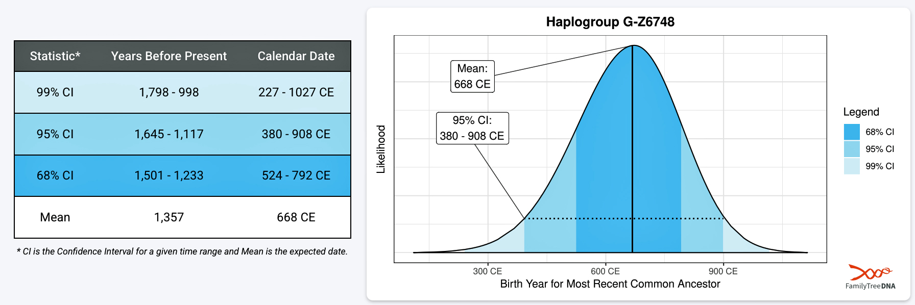
