
This story is a continuation of my focus on the G Haplogroup phylogenetic tree of the Griff(is)(es)(ith) patrilineal line of descent and the migratory route of the Griffis family Y-DNA in the long term genealogical time layer. This story also touches on two historical periods in the migratory path for the family patrilineal line where the lineage experienced two relatively large time gaps between known haplogroups in the ancestors’ European migratory path. Given its length, I have divided the story into two parts.
G Haplogroup European Migration in Context of European Waves of Haplogroup Migration
Illustration one provides a map depicting the general migrations of three successive waves of humans into Europe that formed the genetic ‘melting pot’ of the European population today. The peopling of Europe involved three major demographic waves that reshaped its genetic landscape: indigenous Western Hunter-Gatherers (WHG), Neolithic farmers migrating from Anatolia (Early European Farmers – EEF), and Yamnaya pastoral Western Steppe Herders (WSH) from the Pontic-Caspian region. Each group left distinct genetic markers in mitochondrial (mtDNA) and Y-chromosomal haplogroups, reflecting their origins, migrations, and interactions.
Illustration One: The Three Waves of Human Migration in Europe
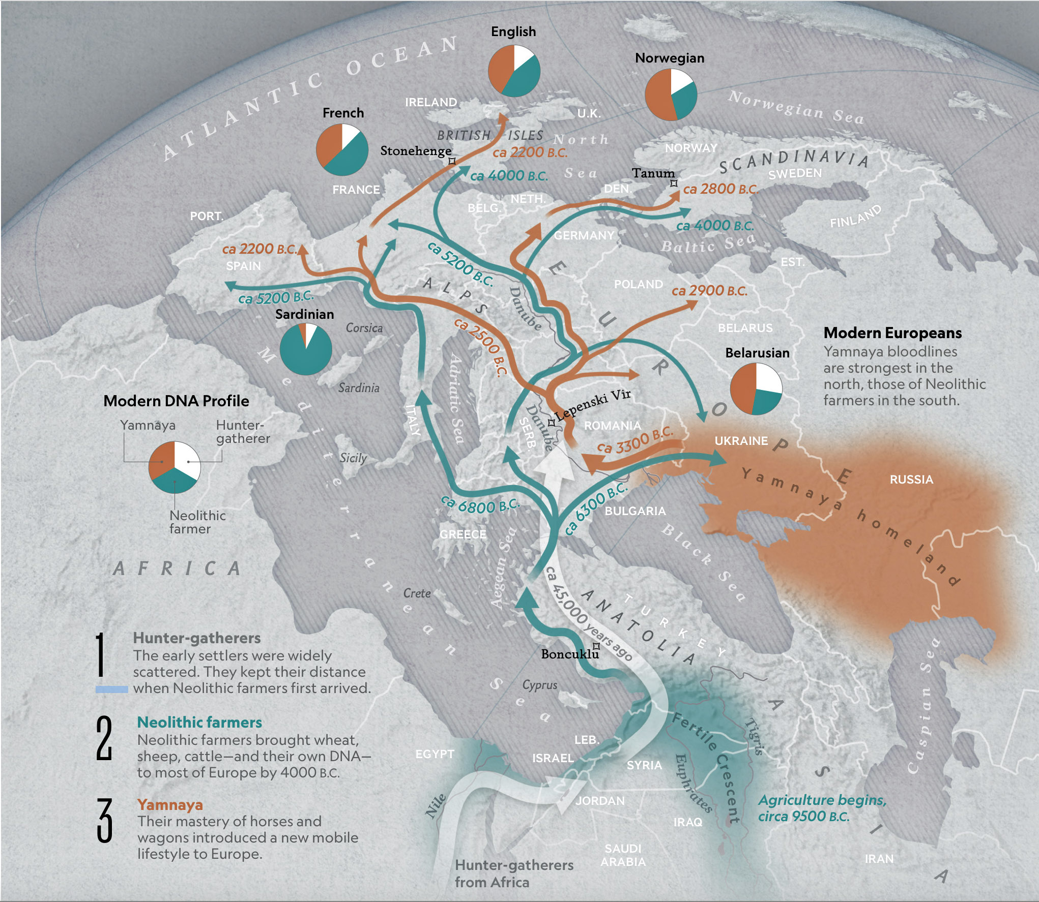
The three waves of European settlement each contributed distinct haplogroup signatures. The WHG left a legacy of haplogroups mtDNA U5 and YDNA I2, while EEF introduced mtDNA N1a and YDNA G2a. The WSH migrations catalyzed a major YDNA chromosomal shift to YDNA R1b/R1a and introduced I, U2, and T1 mtDNA. The mtDNA haplogroup H’s rise to dominance (more than 40 percent in modern Europeans) reflects complex interactions with other groups and was initially rare among EEF. [1] It expanded through the admixture between Steppe groups and Neolithic survivors.
These and other genetic turnovers underscore Europe’s dynamic prehistory, where migration, cultural exchange, and demographic replacement shaped its biological and cultural landscapes. The intersection and admixture of these three waves of genetic YDNA groups influenced and partly explain the shape of the phylogenetic tree associated with the Griff(is)(es)(ith) patrilneal line.
- Western Hunter-Gatherers (WHG)
The WHG populations, present in Europe since the Upper Paleolithic (~45,000–12,000 BCE), carried mtDNA haplogroups U5, U4, and U8, which dominated their genetic profile. These lineages were nearly exclusive to pre-Neolithic foragers, with U5 being the most prevalent (60–90 percent of WHG mtDNA). The absence of haplogroups like H, J, or T in early WHG underscores their genetic distinction from later arrivals. [2]
WHG males primarily belonged to haplogroup I2, particularly subclades like I2a1b, which persisted in isolated pockets into the Neolithic period. [3] Eastern Hunter-Gatherers (EHG), a related but distinct group from Russia, carried R1a and R1b lineages, foreshadowing their later prominence in Steppe populations. [4]
- Early European Farmers (EEF)
Early European Farmers (EEF) from Anatolia introduced a “Neolithic package” of mtDNA haplogroups: N1a, T2, K, J, HV, V, W, and X. [5] N1a, rare in modern Europeans (less than 0.2 percent), was a signature of the Linear Pottery Culture (LBK, ~5500 BCE), reaching 15 percent frequency in early farmers. [6] Haplogroups H and U5, though initially scarce in Anatolian migrants, increased in frequency through admixture with WHG during the Middle Neolithic (approximately 4000 BCE). [7]
The Neolithic farmer migration into Europe, which began around 9,000 years ago, involved significant genetic contributions from populations originating in the Near East. The Y-chromosomal haplogroups associated with these early farmers primarily included G2a and its subclades, which are considered markers of the Neolithic expansion. The G2a haplogroup was predominant among early Neolithic farmers and is strongly associated with the spread of agriculture from the Near East into Europe. [8]
Haplogroup I2a was present in lower frequencies and is thought to represent a legacy of Mesolithic hunter-gatherer populations in Europe. While it was not dominant among Neolithic farmers, it occasionally appeared in mixed contexts, reflecting limited admixture with local hunter-gatherers. [9]
- Western Steppe Herders (WSH) or pastoralists
The WSH Steppe pastoralists associated with the Yamnaya culture (~3300 BCE) introduced novel mtDNA lineages to Europe, including I, U2, and T1, which were absent in preceding populations. [10] These haplogroups, prevalent in Eastern European and Siberian foragers, comprised around 20 percent of Corded Ware Culture (CWC) mtDNA. CWC existed approximately between 3000 BCE and 2350 BE. [11] Later, the Bell Beaker Culture (BBC, about 2800 BCE) exhibited a dramatic shift to haplogroup H (about 48 percent), likely through integration of local farmer ancestry rather than direct Steppe origins. [12]
The Yamnaya expansion marked the rise of R1b-Z2103 and R1a-M417, which replaced roughly 90 percent of preceding farmer Y lineages in Central Europe by 2500 BCE. [13] Corded Ware males were initially R1b-dominant, but R1a-M417 became predominant by 2400 BCE, reflecting dynastic succession or founder effects. [14] In contrast, BBC males carried R1b-L51, a lineage that spread rapidly across Western Europe. [15]
There were some exceptions to this general wave of WSH genetic dominance in mtDNA migratory patterns. In the Eastern Baltic, WSH mtDNA (e.g., U4, U5a) persisted into the Late Neolithic, with only minimal Steppe ancestry (about 15 percent) detected in Corded Ware culture individuals. [16] This contrasts with Central Europe, where Steppe ancestry reached 75 percent. [17] The Narva culture (~4440–4240 BCE) carried haplogroup H without EEF migratory admixture, suggesting a pre-Neolithic haplogroup H presence in rare WHG subgroups. [18]
While Steppe ancestry permeated most of Europe by 2000 BCE, Iberian populations retained higher EEF ancestry (about 50 percent) and elevated the mtDNA haplogroup H frequencies, possibly due to later Bell Beaker migrations from the north. [19] The Basque people, with about 80 percent percent EEF ancestry, exemplify this genetic continuity. [20]
The decline of early European haplogroups like G2a2, which is my patrilineal genetic line of descent, and H2 represented a dramatic genetic replacement event that occurred during the Bronze Age (about 3300 BCE – 1200 BCE). Originally, G2a was the dominant haplogroup among Early European farmers, particularly in the Mediterranean region and Central Europe.
Today, G2a only makes up about 5-10 percent of Mediterranean European populations, with higher frequencies limited to isolated mountainous regions like the Apennines (15-25 percent), Sardinia (12 percent), Cantabria (10 percent), and the Austrian Alps (8 percent). Other regions with notable frequencies include northern Greece (Thessaly), Crete, Asturias (Spain), Auvergne (France), Switzerland, and Cyprus, where percentages approach or exceed 10%. These patterns reflect the survival of Neolithic populations in geographically isolated areas after successive waves of migration and invasion. [21]
While YDNA haplogrops R and I became dominant and the size of G haplogroup ancestors diminished over time, there is a plausible argument that the remaining G haplogroup males became enculturated in Steppe culture and were part of migratory patterns that coincided with the dominant R and I haplogroup males in the Bronze age and later. This absorbtion in successive emerging cultures and social structures resulted in a phylogenetic tree that has fewer branches and long durations between haplogrups.
The Interaction and Admixture of Early Hunter Gatherers and Early European Farmers
“How did the encounter between such disparate peoples unfold? … The answer is: in a kaleidoscope of different ways. There is no clear genetic evidence of interbreeding along the central European route until the LBK farmers reached the Rhine. And yet the groups mixed in other ways—potentially right from the beginning.“ [22]
Paleogenetic and anthropological studies revealed that early European farmers initially mixed minimally with local hunter-gatherers. However, during the Middle Neolithic period (6000 – 4000 BCE) [23], there was increased mixing predominantly involving hunter-gatherer males and farmer females. This pattern suggests a social structure where hunter-gatherer men integrated into farming communities, potentially reflecting power dynamics or social stratification. [24] The near absence of WHG-derived Y lineages (e.g., I2) in early Neolithic communities highlights strict patrilocal practices. [25] Patrilocal practices, in social anthropology, refer to a residence pattern where a married couple lives with or near the husband’s family, often his parents, after marriage. [26]
Previous analyses had suggested that the EEF were genetically different from other human groups from that time. A number of paleogenomic studies have claimed that the first farmers of Anatolia and Europe emerged from a population admixed between hunter-gatherers from Europe and the Near East. The mixing process started around 14,000 years ago, which was followed by a period of extreme genetic differentiation lasting several thousand years. [27]
Various studies have shown regional variations in how farming spread based on haplogroups admixture. In Britain, evidence suggests Aegean migrants virtually replaced the existing hunter-gatherer population with limited interbreeding around 4000 BCE. [28] By contrast, Baltic hunter-gatherers acquired farming knowledge through cultural exchange rather than genetic admixture, maintaining genetic continuity despite adopting new technologies. [29] In the Lower Danube Basin, which is the path the Griff(is)(es)(ith) ancestors had taken, paleogenomic evidence has revealed multi-generational mixing between Neolithic farmers and Mesolithic hunter-gatherers [30] A study by Joaquim Fort and others found that despite differences in dispersal patterns, the percentage of farmers who interbred with hunter-gatherers was remarkably consistent. [31]
The Continental Route of G Haplogroup Migration
Neolithic farmers along the Continental Route, which is the route taken by Griffis)(es)(ith) ancestors, had an effective population size approximately five times larger than contemporaneous hunter-gatherer groups. [32] This demographic advantage, combined with technological innovations like polished stone tools and pottery, enabled rapid territorial expansion. [33] These findings support a model of demic diffusion (population replacement) rather than cultural transmission alone. [34]
“The farmers reached the new continent by two routes: in boats via the Mediterranean and on foot along the Danube River from the Balkans into central Europe. Radiocarbon dating of archaeological sites revealed that by about 7,500 years ago, Danubian farmers were building villages in the Carpathian Basin—modern-day Slovakia, Hungary and Romania—and there they began creating a pottery culture. Archaeologists call it the Linear Pottery culture (LBK, by its German acronym, for Linearbandkeramik).
“Traveling rapidly westward across the fertile plains of what is now Germany, the LBK farmers reached the Rhine within just a few centuries, around 7,300 years ago. (See illustration two.) Fine-grained analysis of the evolution of pottery styles, along with radiocarbon dating, suggests that they practiced a form of leapfrog colonization. They took “stepwise movements with sometimes hundreds of kilometers covered, and then the landscape in between filled up,”…” [35]
Illustration Two: Major Rivers in Europe and the Path of the Griff(is)(es)(ith) YDNA Haplogroup Migration
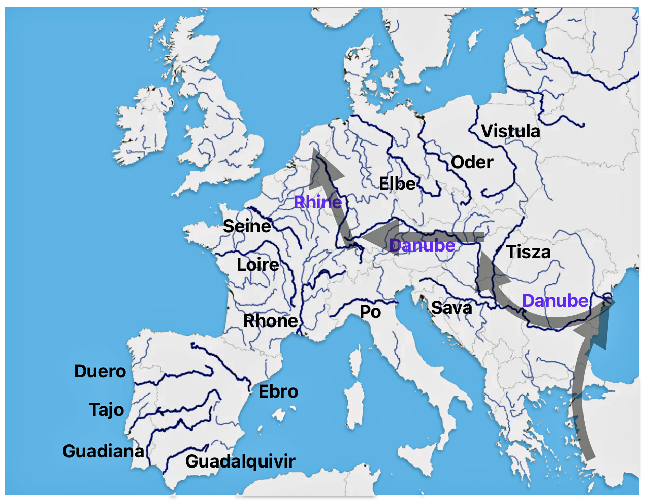
https://www.reddit.com/r/MapPorn/comments/jzn9y0/rivers_of_europe/#lightbox
Early Neolithic farmers along the Continental Route initially occupied ecological niches among the loess plains of river valleys distinct from hunter-gatherer territories (forested uplands). Isotopic analyses of LBK burials indicate diets heavily reliant on terrestrial protein (cattle and wheat), contrasting with hunter-gatherers’ marine/freshwater resources. [36] This ecological partitioning limited direct competition but also minimized genetic exchange during the LBK’s formative phase. [37]
By 5200 BCE, archaeological and genetic evidence points to increased interaction between the indigenous hunter gatherers and the farmers that migrated along the Dunube and Rhine and other tributaries:
- Material cultural exchanges: Hunter-gatherer lithic styles (e.g., microliths) appear in LBK contexts. [38]
- Genetic admixture: Analyses of ancient remains of Late LBK individuals reflect up to 15 percent hunter-gatherer genetic ancestry, with higher proportions in frontier zones like the North European Plain. [39]
- Subsistence shifts: Some LBK communities incorporated wild game (aurochs, red deer) into their diets, reflecting adaptive hybridization. [40]
This “resurgence” of hunter-gatherer genetic influence suggests that indigenous populations were not wholly displaced but gradually integrated into expanding agricultural societies. Before the disappearance of hunter-gatherer lifeways in Europe, farmers and foragers coexisted for many generations and in certain instances for thousands of years. [41]
The Starčevo culture’s expansion into the Carpathian Basin (6000–5400 BCE) marked the first phase of the Continental Migratory Route. (See illustration two regarding the geographical cultural areas at the time.) These early farmers practiced small-scale agriculture, relying on emmer wheat and domesticated cattle, while maintaining limited contact with local hunter-gatherers. [42] Archaeo-botanical evidence from sites like Alsónyék-Bátaszék (Hungary) shows a gradual shift from wild to domesticated plant use, suggesting a transitional economy. However, genetic data from Starčevo-associated individuals reveal minimal hunter-gatherer ancestry (less then 5 percent), indicating that early interactions were largely cultural rather than biological. [43]
Illustration Two: European Cultures Between 5000 BCE and 4500 BCE
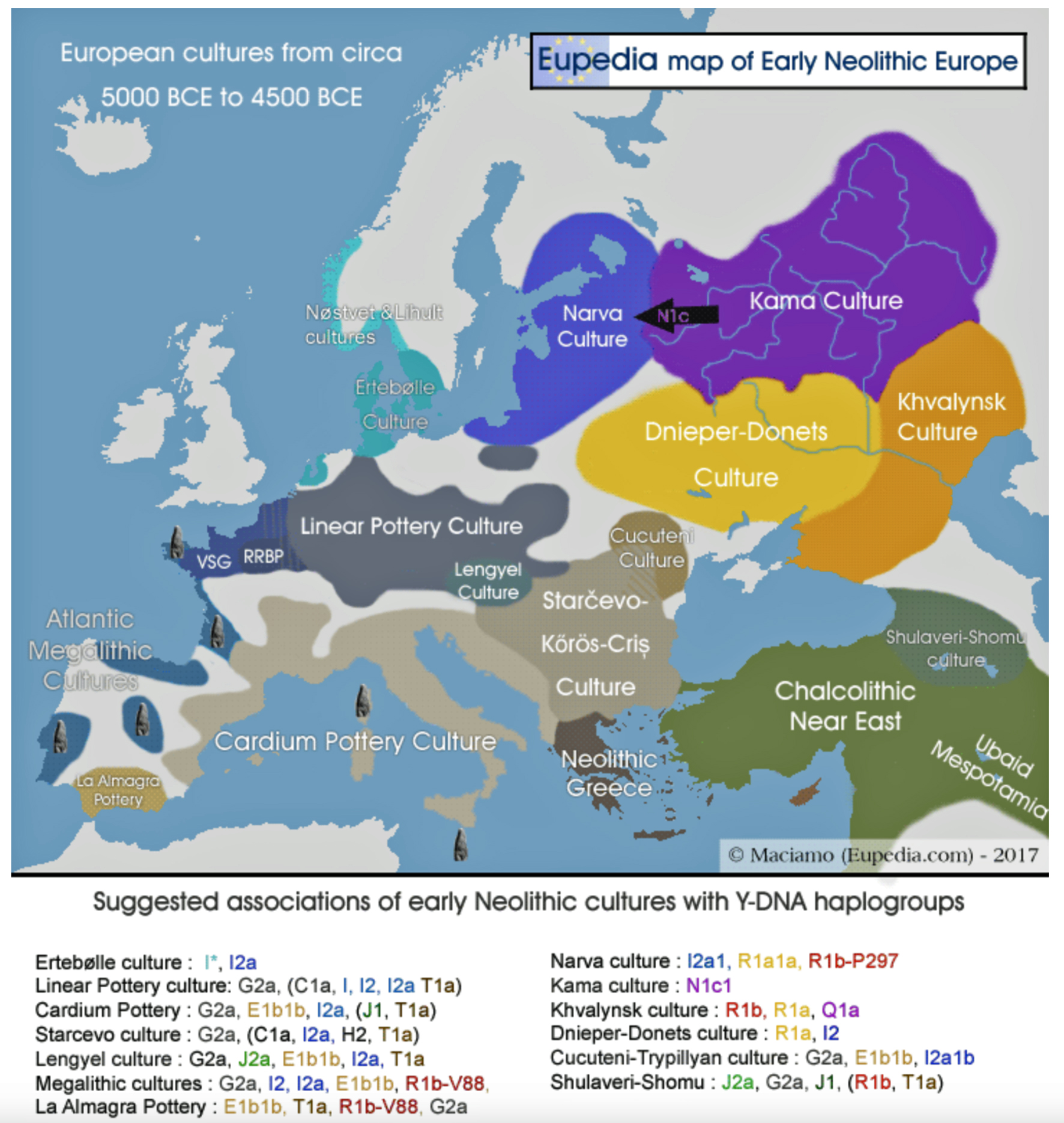
Around 5500 BCE, the Linear Pottery Culture (LBK) emerged in Transdanubia (western Hungary), catalyzing the Neolithic’s rapid dispersal into Central Europe. The interaction between Starčevo farmers and local hunter-gatherers in Transdanubia (Hungary) produced the LBKT (LBK Transdanubia), a hybrid culture blending ceramic traditions and subsistence strategies. Genetic data from Vráble-Veľké Lehemby (Slovakia) reveal that LBKT individuals retained about 95 percent of Anatolian ancestry, underscoring limited initial admixture. [44]
Characterized by distinctive incised pottery and longhouse settlements, LBK communities expanded at an average rate of 1 to 1.3 kilometers per year, reaching the Rhine Valley by 5300 BCE and the Paris Basin by 5000 BCE. [45] This “wave of advance” was facilitated by a combination of ecological and social cultural influences:
- Loess soil exploitation: Fertile, wind-deposited soils supported intensive cereal cultivation. [46]
- Riverine networks: The Danube, Elbe, and Rhine provided transport routes and ecological connectivity for the migratory routes of the G haplogroup. [47]
- Social cohesion: LBK settlements exhibited uniform material culture, suggesting strong cultural transmission. [48]
Genetic studies of LBK populations reveal a near-complete absence of hunter-gatherer mitochondrial lineages (e.g., U5b), reinforcing the model of farmer-led migration. [49] However, sporadic admixture between the two is detectable in later phases, with hunter-gatherer ancestry rising to about 10 percent in Middle Neolithic groups. [50]
The continental route of Neolithic expansion was not a monolithic “wave of advance” but a complex process shaped by demographic, ecological, and cultural exchange. A demic diffusion dominated the early phases, with farmer migrations driven by demographic pressures and ecological preferences. Admixture increased regionally over time, reflecting an adaptive integration of hunter-gatherer populations with the early western farmers.
The Interaction and Admixture of Early European Farmers and the Steppe Pastoralists
The interaction between haplogroups G2a and R in Europe represents one of the most significant demographic transitions in human prehistory. The Neolithic G2a-bearing farmers who spread agriculture across Europe experienced a dramatic population replacement during the Bronze Age with the expansion of R1b lineages from the east. This transition was not a simple replacement, however, as evidenced by regional persistence of G2a in certain areas and the complex patterns of admixture seen in both ancient and modern populations.
Approximately 5,000 years ago (3000-2500 BCE) a remarkable migration from the Eurasian steppe dramatically transformed the genetic and linguistic landscape of prehistoric Europe. The Yamnaya culture, a group of nomadic pastoralists from what is now Russia and Ukraine, swept westward into Europe, bringing with them not only new technologies and cultural practices but also the ancestral forms of many modern European languages. [51]
Illustration three depicts the various migratory paths of the Steppe Pastoralists. The black lined route depicts the eastward migration starting east of Carpatian mountains as found in the Corded Ware culture, transforming into the successive cultures: Fatyanovo–Balanovo culture (2800 BCE), the Abashevo (2200 BCE), the Sintashta (2100-1900 BCE)-> Andronovo (1900-1700 BCE) and Indo-Aryans. The initial eastward migration around 3000 BCE, from the black circle on the map, started with the Afanasievo culture, possibly Proto-Tocharian culture. The north-westward migrations, around 2900 BCE) carrying Corded Ware culture, transforming into the Bell Beaker culture. The westward migration west of Carpatians continued into Hungary as Yamnaya, transforming into Bell Beaker culture. [52]
Illustration Three: Migration of Steppe Pastoralists
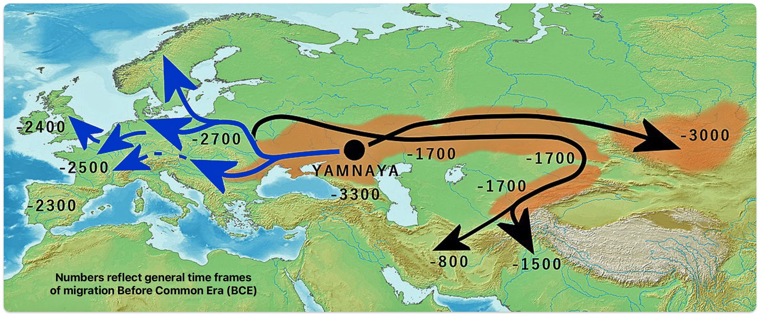
Genetic and archaeological research has provided compelling evidence for this migration and its profound impact on European prehistory. The Yamnaya were an early Bronze Age culture that emerged from the vast grasslands of the Eurasian steppe between the Southern Bug, Dniester, and Ural rivers in present-day Ukraine and Russia around 3300 BCE. They developed from an earlier population known as the Caucasus-Lower Volga (CLV) group, who lived between the Volga River and the Caucasus Mountains approximately 6,500 years ago. [53]
Archaeological and genetic evidence indicates the Yamnaya were not a genetically homogeneous population but rather a mixed group. Their genetic makeup suggests that the leading clans were of Eastern European hunter-gatherer (EHG) and Western European hunter-gatherer (WHG) paternal origin. [54] Additionally, between 35 percent and 50 percent of Yamnaya ancestry came from the South Caucasus-Zagros area, establishing a connection between “the Proto-Indo-European-speaking Yamnaya with the speakers of Anatolian languages“. [55]
The Yamnaya developed significant technological innovations that facilitated their mobile lifestyle and subsequent expansion. They were likely among the first people to herd on horseback, a revolutionary advancement that increased mobility and range. [56] They utilized wagons for transportation, allowing movement of goods and families across vast distances. [57] They brought metallurgy skills to Europe, contributing to technological advancement. [58] They were skilled at “harvesting the bioenergy of the Eurasian grasslands” through pastoral nomadism. [59]
One of the most striking aspects of the Yamnaya migration was its gender imbalance. Genetic studies suggest this was a predominantly male movement. The contrasting patterns of sex-specific migration suggest fundamentally different types of interactions between migrating and local populations during the the Neolithic expansion of early farmers and the Steppe migration. These findings help explain cultural transitions observed in the archaeological record, including changes in burial practices, technology, and social structures: [60]
- The Neolithic expansion likely involved the movement of entire family units, suggesting a more gradual and integrative cultural spread.
- The Steppe migration appears to have been a more male-dominated process, possibly involving male warriors or herders who then sought wives from local European farming populations.
- Researchers have indicated an extremetly skewed sex ratio associated with the Steppe migration, estimating approximately 5-14 migrating males for every migrating female.
- The research points to ongoing, primarily male migration from the Steppe to Central Europe over multiple generations.
- The male-biased Steppe migration pattern was possibly connected to new technologies, particularly horses and chariots, and conquest strategies.
This shift represents not just a change in genetic markers but reflects profound differences in social organization, cultural practices, and technological adaptations that gave the R haplogroup populations competitive advantages.
Neolithic farming communities associated with haplogroup G, particularly G2a, established Europe’s first agricultural societies. Archaeological and genetic studies have revealed important aspects of their social organization: [61]
- They were organized into patrilocal and patrilineal communities with stable family structures.
- Evidence from sites like Gurgy ‘les Noisats’ in France shows these communities consisted of genetically connected pedigrees spanning multiple generations.
- They practiced female exogamy (women marrying outside their group) and formed monogamous reproductive partnerships.
- Their settlement patterns suggest relatively stable health conditions that supported high fertility rates.
- These societies exhibited some social stratification, though perhaps less pronounced than later Indo-European groups.
The G2a farmers’ social structure prioritized stability and continuity, which aligned perfectly with their sedentary agricultural lifestyle. While functional, this stability may have made them less adaptable to competition with more militarily organized societies.
In contrast, the R haplogroup pastoralists from the Eurasian steppes developed a markedly different social configuration: [62]
- Their social structure was strongly patriarchal and hierarchical with distinct social classes including priests, warriors, chiefs, commoners, and slaves.
- Their socieities oncentrated wealth and power in male lineages and Increased social inequality linked to patrilineal inheritance systems.
- Their social organization particularly was effective for warfare and expansion.
- Young males were initiated into warrior-bands called kóryos, living by hunting, raiding, and pillaging other communities.
- Their society was organized around patron-client relationships that facilitated military endeavors.
- Exogamy practices allowed for the incorporation of foreign women into their societies, enabling demographic growth even in conquest scenarios.
This warrior-centric social organization gave R haplogroup populations significant advantages in conflict situations. The kóryos tradition in particular appears to have been a powerful vehicle for expansion, as these groups of young warriors could effectively raid sedentary farming communities.
Within just a few hundred years, the Yamnaya contributed to at least half of central Europeans’ genetic ancestry. [63] Their genetic impact varied geographically, with Northern Europeans showing stronger Yamnaya ancestry than Southern Europeans. It has been estimted that the Yamnaya genetic contribution in modern Eastern Europeans ranges from roughly 47 percent among Russians to 43 percent in Ukrainians, with Finland having the highest Yamnaya contribution in all of Europe at 50 percent. [64]
The genetic history revealed through these Y-chromosome lineages aligns with archaeological evidence for cultural transitions and provides insights into the formation of the modern European genetic landscape. While male lineages show evidence of substantial replacement, autosomal DNA reveals a more nuanced picture of admixture between different ancestral populations. This complex interplay between replacement and admixture has shaped the genetic diversity of Europe today, creating a mosaic of ancestry that reflects thousands of years of human migration, interaction, and cultural change.
The G Haplogroup Phylogenetic Tree in the Long Term Genealogical Time Layer
The shape and nature of the G haplogroup phylogenetic tree is for the most part long and narrow. The particular branch of the G haplogroup, which includes the migratory path of the Griff(is)(es)(ith) family, is characterized, with few exceptions, as a haplogroup with few subclades spread over a long periods of time.
Haplogroup G’s current European distribution is characterized by overall low frequency across Europe punctuated by geographically isolated regions of higher concentration. The haplogroup is historically associated with early Neolithic agricultural expansions from the Near East into Europe via the northern Mediterranean coastline (the Mediterranean route) and the inland route, traversing the Balkans and central Europe via the Danube and Rhine rivers and other tributaries.
The phylogenetic tree of haplogroup G in general reveals a complex history characterized by an early divergence into two major branches (G1 and G2), followed by subsequent diversification into geographically specific subclades. Its development spans from approximately 48,500 years ago to much more recent times, with significant expansion events occurring after the Last Glacial Maximum (26,000 – 20,000 years ago) and during the Neolithic period. ( 7000–1700 BCE ). [65]
The tree’s shape reflects multiple migration events and population bottlenecks rather than simple migration dispersal, with different subclades showing distinct geographic patterns. The higher diversity near the proposed homeland in West Asia/Middle East and the more restricted distribution of specific subclades in peripheral regions supports a model of outward migration from this central zone, with subsequent isolation and local evolution in different geographic regions. [66]
Haplogroup G (M201) emerged as one of two primary branches from the parent haplogroup GHIJK, with HIJK being its sibling clade. The overall shape of the G haplogroup tree can be characterized as having two primary branches that formed early in its history, with subsequent diversification into numerous subclades displaying strong geographical specificity.
The haplogroup G phylogenetic tree splits into two fundamental branches: the G1 (M285, M342) haplogroups which is less common globally but shows significant presence in specific regions and the G2 (P287) haplogroups which is the predominant branch containing most G lineages. [67]
The Significance of G-P15 and G-P303 Haplogroups
Haplogroup G2 further divides into: G2a (P15) which is the most widespread subclade in Europe and haplogroup G2b (M3115) which is found from the Middle East to Pakistan. Illustration four below provides a depiction of a phylogenetic tree for G-P15.
Illustration Four: Phylogenetic trees of haplogroup G2a and Haplogroup G2a-L140 (Shaded Arrows Depict Griff(is)(es)(ith) Line of Descent)
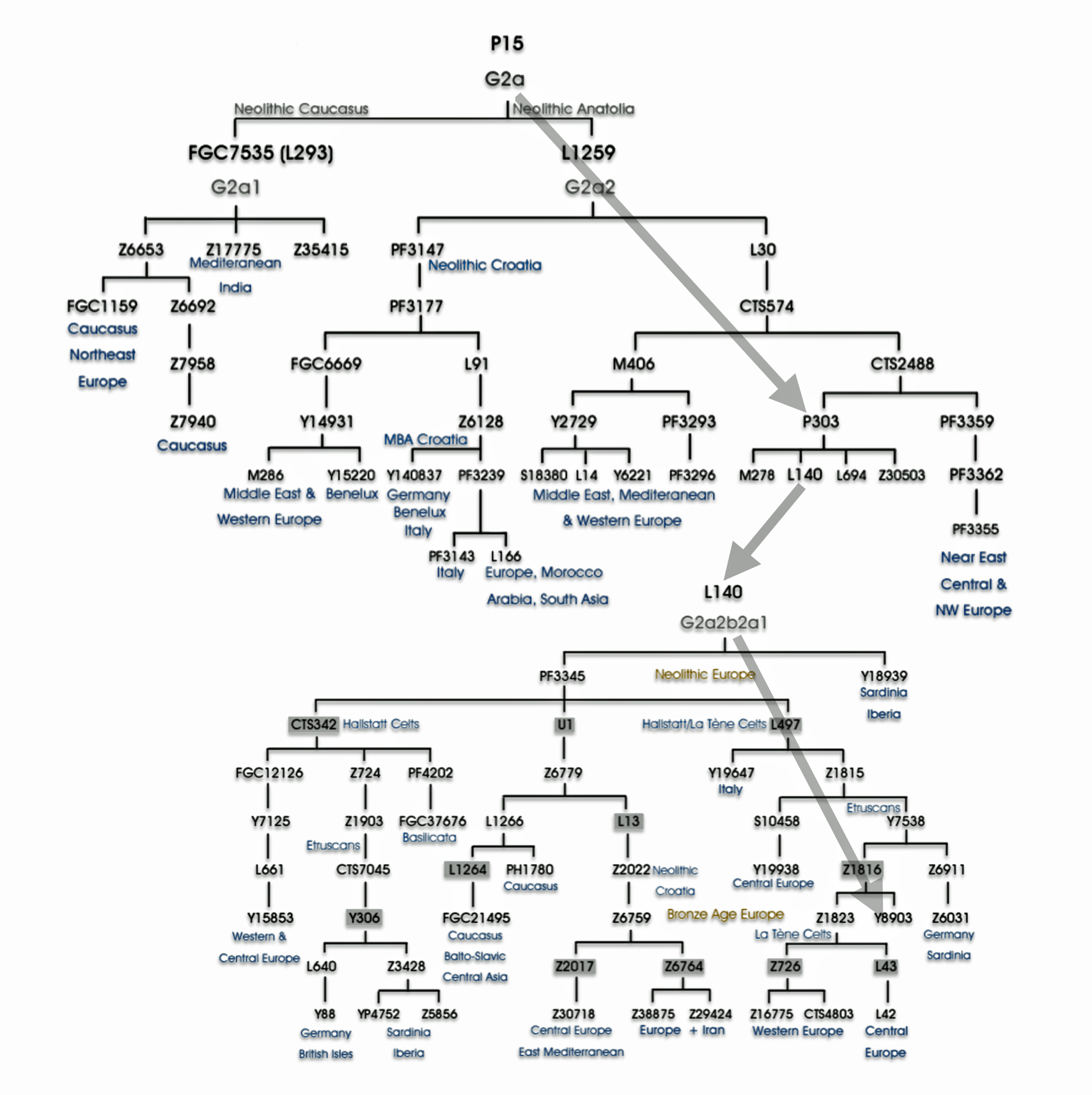
“(A) predominance or high frequency of the Y-chromosome haplogroup G- P15 in representatives of various Neolithic archaeological cultures of Europe with a pronounced decrease or complete absence in the subsequent cultures confirms the hypothesis on Neolithic expansion of Anatolian/Middle Eastern farmers toward Western Europe, which was followed by their displacement by such steppe ancestors as pro-Indo-European steppe nomads. [68]
Illustration Five: Archaeological Sites with Detected Y-Chromosome Haplogroup G-P15 Across Europe
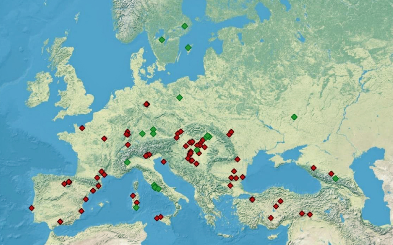
Recent genetic studies have enhanced the understanding of G2a’s structure with several defined subclades showing geographic specificity for each of the major subclades. For example, haplogroup G2a-L140, who is a genetic ancestor of the Griff(is)(es)(ith) family line, and G2a-M406 predominate in northern and western Europe.
This genetic lineage offers insights into prehistoric human migrations, early agricultural expansions, and the complex genetic tapestry connecting populations across Europe, the Caucasus, and the Middle East. The overall coalescent age estimate for G-P303 is approximately 12,600 years ago, placing its emergence in the early post-glacial period. (The coalescent age is essentially the time to the most recent common ancestor (tMRCA) of a set of gene copies.) This timing is significant as it corresponds to a critical transition period between hunter-gatherer societies and the emergence of early agricultural communities.
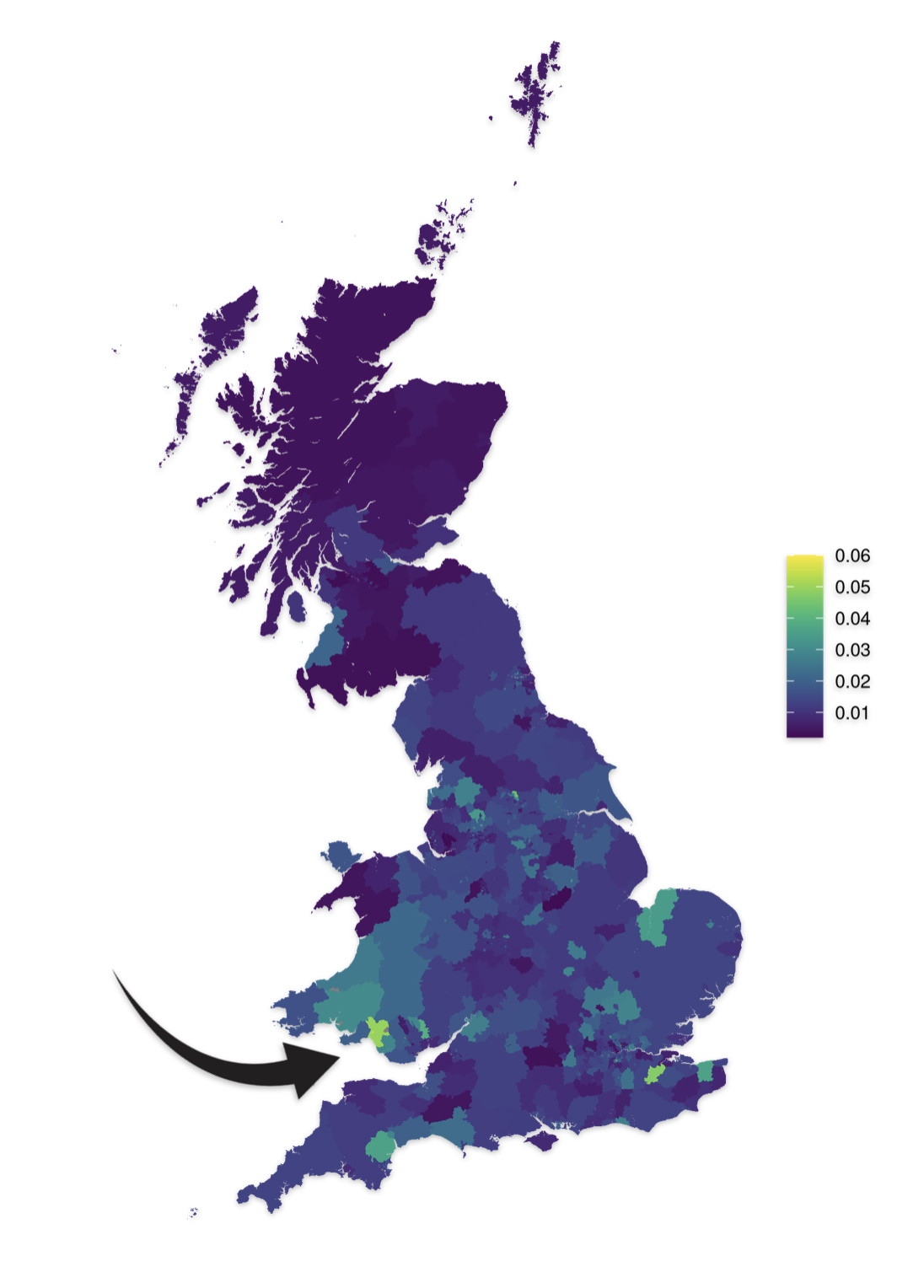
Haplogroup G-P303 defines the most frequent and widespread G subclade globally. In Europe, G-P303 definable subgroups make up a majority of Haplogroup G persons west of Russia and the Black Sea, and small numbers are also found in North Africa. The percentage of haplogroup G among available samples from Wales is overwhelmingly G-P303. Such a high percentage is not found in nearby England, Scotland or Ireland. [69]
Table one below provides a comparison of specific YDNA Short Tandem Repeats (STRs), also known as microsatellites, that are associated with the G-P303 haplogrup. The table provides a comparison of these values with my test results. STRs are short, repetitive DNA sequences (typically 2-6 base pairs) that are found throughout the genome, and the number of repeats varies between individuals, making them useful for DNA identification and analysis. STR values represent the number of times a short, repeating DNA sequence occurs at a specific location (locus) on a chromosome.
“All G-P303 men carry the P303 or S135 SNP Y-DNA mutation. There are also some short tandem repeat (STR) findings among G-P303 men which help in subgrouping them. Many of the men have an unusual value of 13 for marker DYS388, and some have 9 at DYS568. STR marker oddities are often different in each G-P303 subgroup, and characteristic marker values can vary by subgroup. Often the values of STR markers DYS391, DYS392 and DYS393, however, are respectively 10, 11 and 14 or some slight variation on these for all G-P303 men.“ [70]
Table One : My Short Tandem repeats STR Values Associated with G-P303
| Designated STR Y Chromosome Segment (DYS) | STR DYS Values Associated with G-P303 | My STR DYS Values Associated with G-P303 |
|---|---|---|
| YS388 | 13 | 13 |
| DYS391 | 10 | 10 |
| DYS392 | 11 | 11 |
| DYS393 | 14 | 15 |
| DYS594 (Welsh Association) | 12 | 11 |
The table indicates that my test results are identical to or one value off of the values associated with the G-P303 STR configuration.
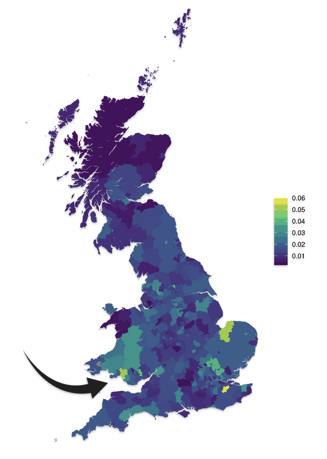
A 2022 study systematically assessed the association between genetic variation in the male-specific region of the Y chromosome (MSY) and cardiovascular disease outcomes in Great Britain. While the primary finding of the study showed little evidence for an effect of any MSY haplogroup on cardiovascular risk in participants, an important secondary finding was that Y chromosome haplogroups carried by the British UK Biobank sampled individuals demonstrate a strong geographic structuring across Great Britain. [72]

This extensive analysis included up to 152,186 unrelated, genomically British individuals from UK Biobank. The Biobank has data on the whole genome sequencing for 500,000 participants, whole exome sequencing for 470,000 participants, genotyping (800,000 genome-wide variants and imputation to 90 million variants).
The prevalence of male-specific region of the Y chromosome haplogroups was plotted by place of birth in successively larger areas with at least 100 individuals, from wards and electoral divisions, to local authorities, to regions of England and the nations of Great Britain. Examples of geographic structuring of Y chromosome variation by place of birth of genetically British men from UK Biobank were depicted in maps of 90 haplogroups in the study. [73]
As reflected in illustrations five and six for haplogroups G-M201 and G-P15 respectively, there is a small prevalence of the G haplgroup in sourthern Wales where it has been hypothesized where the Griff(is)(es)(ith) family emigrated from when traveling to the American colonies.
Illustration Five: G-M201 Prevalence by Geographic Area
https://datashare.ed.ac.uk/bitstream/handle/10283/4450/st004_03_G_M201_birth.png?sequence=13&isAllowed=y
Illustration Six: G-P15 Prevalance by Geographic Area
https://datashare.ed.ac.uk/bitstream/handle/10283/4450/st004_03_G2a_P15S_birth.png?sequence=14&isAllowed=y
The haplogroup G-L497 lineage, which is also a genetic ancestor of the Griff(is)(es)(ith) line. It belongs to the larger G2a branch and specifically the P303 subclade. G-L497 is a significant Y-chromosome haplogroup that represents one of the major European branches of haplogroup G. Most carriers, such as myself, have a distinctive value of 13 at the DYS388 marker (see table one above). [74]
G-L497’s subclades (e.g., L91, P303) correlate with specific migration waves. For instance, G2a-P303 spread into Central Europe during the Neolithic. G-L497 shows a distinct European concentration, particularly along the Rhine River and in alpine regions. The haplogroup reaches its highest frequencies in the Tyrolean Alps [75], where some valleys show concentrations above 40 percent. It is commonly found among populations in the United Kingdom and Ireland. [76] The G-L497 hsaplogroup is also found in various parts of Europe. High percentagesare found in northwestern Europe, with notable frequencies in Switzerland (74%), Spain (60%),France (58%), and Germany (57%). [77]
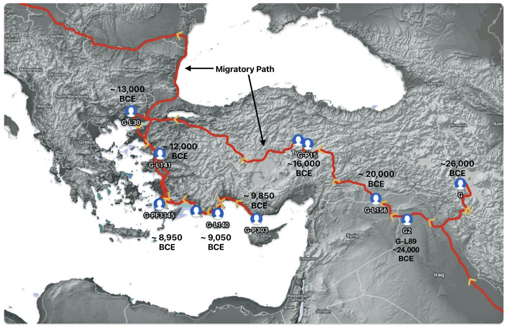
Illustration seven depicts the estimated early migratory path of ancestors genetically related to my G-Y132505 terminal haplogroup prior to migrating westward into Europe. The map depicts selected haplogroup subclades between G-M201, the begining of the G haplogroup (~26000 BCE) and G-L140 (~9050 BCE). It is noteworthy that for approximately 17,000 years, the YDNA G haplogroup lineage was located in the West Asia/Middle East area known as Anatolia. Anatolia, also known as Asia Minor, is the peninsula of land that today constitutes the Asian portion of Turkey.
Illustration Seven: Estimated Early Migratory Path of Griff(is)(es)(ith YDNA Lineage – 26000 BCE to 8950 BCE
Griff(is)(es)(ith) YDNA Phylogentic Line
Table Two provides the YDNA ancestral path of the Griff(is)(es)(ith) line from most recent haplogroup (G-BY211678) that started around 1400 CE to the distant past (Haplogroup A ). With the exception of four haplogroups, each haplogroup had two or three genetic decscendants that continued the genetic YDNA line. Below are explanations for each of the descriptive characteristics associated with each haplogroup.
Explanation of Columns in Table One
| Column | Description |
|---|---|
| Haplogroup | The name of an ancestral haplogroup. |
| Age Estimate of MRCA Brith | The estimated birth date of the ancestor that is associated with the unique SNP mutation that is associated with the haplogroup. |
| Time Passed from Prior Haplogroup | Time elapsed between an haplogroup and its immediate ancestral haplogroup. |
| Number of Phylogenetic Subclades | Number of Phylogenetic subclades provides an indicator to esitmate the relative expansion of the subclade. A large number indicates a rapid expansion event. |
| Number of SNP Variants | If a haplogroup has many associated SNP variants, it suggests a greater level of genetic diversity and potential for sub-branching within that haplogroup, indicating a longer history and more complex evolutionary path. The number of sub-branches is, however, dependent upon archeaological and modern day DNA testing discoveries. |
Table Two: Genetic Ancestral Path for My Terminal Haplogroup G-Y211678
| Haplogroup | Age Estimate of MRCA Birth | Time Passed from Prior Haplogroup (Years) | Number of Phylogenetic Subclades | Number of SNP Variants |
|---|---|---|---|---|
| G-BY211678 | 1400 CE | 300 | 2 | 3 |
| G-Y132505 | 1100 CE | 150 | 4 | 2 |
| G-Z40857 | 950 CE | 250 | 4 | 5 |
| G-Y38335 | 700 CE | < 100 | 2 | 2 |
| G-Z6748 | 650 CE | 2,850 | 2 | 29 |
| G-FGC7516 | 2200 BCE | < 100 | 6 | 1 |
| G-FGC477 | 2250 BCE | 300 | 2 | 1 |
| G-Z727 | 2550 BCE | 550 | 3 | 8 |
| G-Z1817 | 3100 BCE | 850 | 2 | 10 |
| G-Z6901 | 3950 BCE | 650 | 1 | 5 |
| G-Z1900 | 4600 BCE | 300 | 2 | 4 |
| G-CTS9737 | 4900 BCE | 600 | 1 | 9 |
| G-L497 | 5500 BCE | 3,450 | 2 | 48 |
| G-PF3345 | 8950 BCE | < 100 | 11 | 1 |
| G-Z3065 | 8950 BCE | < 100 | 2 | 2 |
| G-PF3346 | 9000 BCE | < 100 | 3 | 1 |
| G-L140 | 9050 BCE | 800 | 3 | 14 |
| G-P303 | 9850 BCE | 2,150 | 3 | 38 |
| G-L141 | 12,000 BCE | 1,000 | 2 | 14 |
| G-L30 | 13,000 BCE | 3,000 | 2 | 47 |
| G-L1259 | 16,000 BCE | < 1,000 | 2 | 7 |
| G-P15 | 16,000 BCE | 4,000 | 2 | 56 |
| G-L156 | 20,000 BCE | 4,000 | 2 | 62 |
| G-L89 (G2) | 24,000 BCE | 2,000 | 2 | 32 |
| G-M201 (G) | 26,000 BCE | 20,000 | 2 | 324 |
| GHIJK-F1329 | 46,000 BCE | 1,000 | 2 | |
| F-M89 | 47,000 BCE | 16,000 | 2 | |
| CF-P143 | 63,000 BCE | 1,000 | 2 | |
| CT-M168 | 64,000 BCE | 22,000 | 2 | |
| BT-M42 | 86,000 BCE | 35,000 | 2 | |
| A-V221 (A1b) | 121,000 BCE | 5,000 | 2 | |
| A-V168 (A1) | 126,000 BCE | 6,000 | 2 | |
| A-L1090 (A0T) | 152,000 BCE | 80,000 | 2 | |
| A-PR2921 (Y-Adam) | 232,000 BCE | 136,000 | 2 | |
| A000-T(Neanderthal Divergence) | 368,000 BCE | 337,000 | 2 | |
| A-0000 (Denisovan divergence) | 705,000 BCE |
If attention is focused on haplogroups that are after G-L140 (~9050 BCE), there are two notable gaps between haplogroups or most common recent ancestors in the migratory chain.
- The 3,500 year Gap between G-PF3345 and G-L497: The common ancestor born around 8550 BCE, associated with the haplogroup G-PF3345, had eleven surviving descendants. The next common ancestor was associated with the G-L497 haplogroup about 3,500 years later. The time that passed from the prior ancestor to G-PF3345 was less than 100 years.
- The 2,850 year Gap between G-FGC7516 and G-Z6748: The other common ancestor born around 2200 BCE, associated with haplogroup G-FGC477, had 6 surviving descendants and the prior ancestor was less than 100 years. The next genetic ancestor was associated with the genetic SNP mutation defining the G-Z6748 haplogroup 2,850 years later. Similar to haplogroup G-PF3345, the preceding genetic ancestor to G-FGC7516 was less than 100 years .
Illustration Eight depicts these two gaps in a map of the estimated migration path of the Griff(is)(es)(ith) patrilineal line. The map depicts various haplogroups along an estimated migratory path for the patrilineal family line.
A dotted arrow connects haplogroup G-PF3345 with haplogroup G-L497. As reflected in the illustration, there a large time gap between the two common descendants. It is also evident that there are no other known, documented G haplogroup descendants that migrated up the western coast of the Black sea and moved westward following the Danube River to an approximate area presently known as Tyrol, Austria. It is in this general area that the ancestor associated with the G-L497 haplogroup was born. [78]
Illustration Eight: Highlighted Haplogroup Gaps in Griff(is)(es)(ith) Migratoy Path
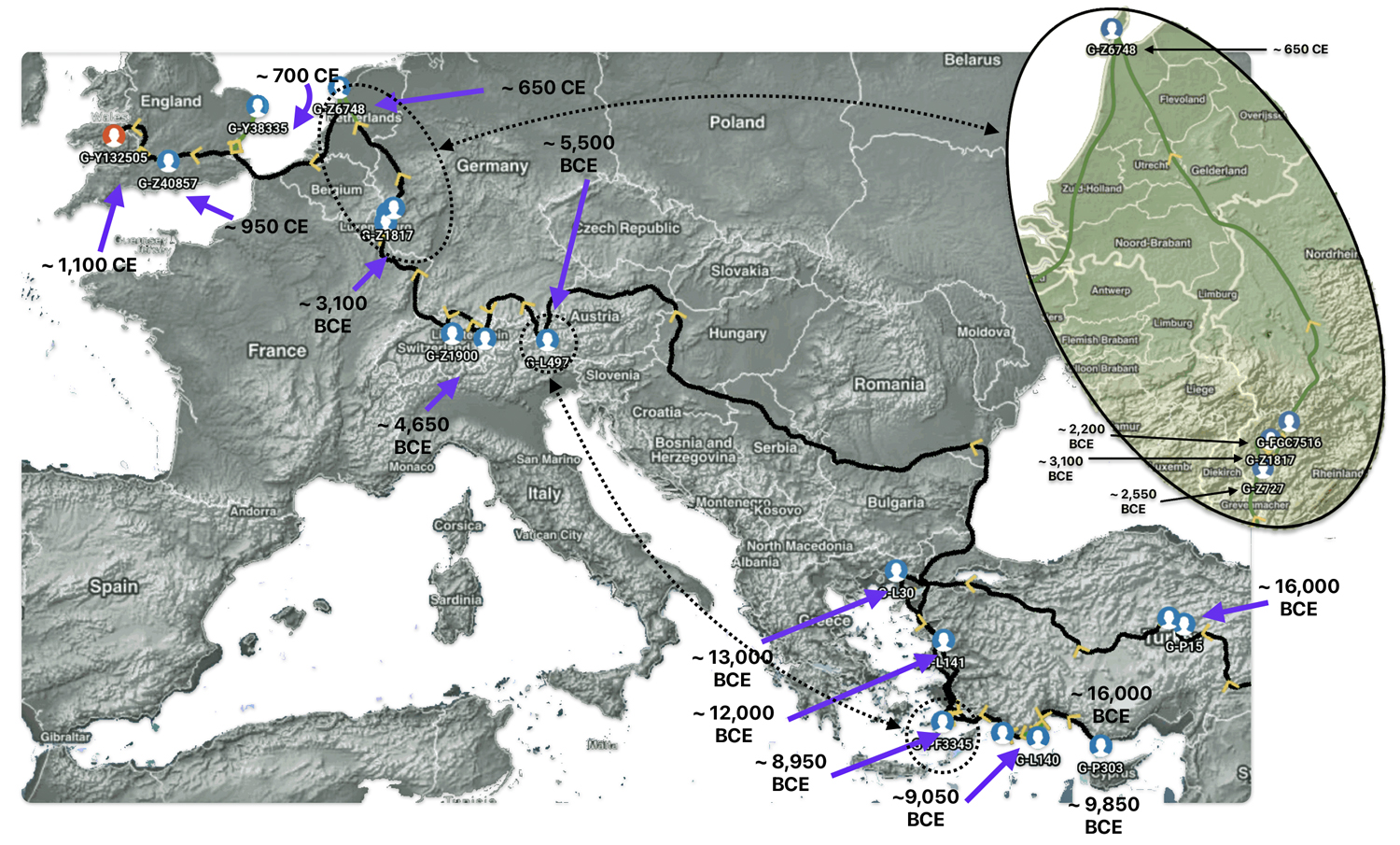
Between roughly 8950 BCE and 5500 BCE, the Griff(is)(es)(ith) family paternal ancestral path was a mystery. Based on geographical and environmental data, it would appear that the migratory path followed the western outline of the Back Sea and continued westward along the second longest river in Europe, what is now known as the Danube River. During this time period the haplogroup path and phylogenetic tree of descendants appears to have been long and narrow.
The other major gap between haplogroups G-FGC7516 and GZ6748 is depicted in illustration nine by an enlarged area of the map in illustration eight. The second phylogenetic gap corresponds with a northward migratory path that is found near modern day Luxemburg and Western Germany.
Illustration Nine: Estimated Migratory Path Between G-FGC7516 and G-Z6748
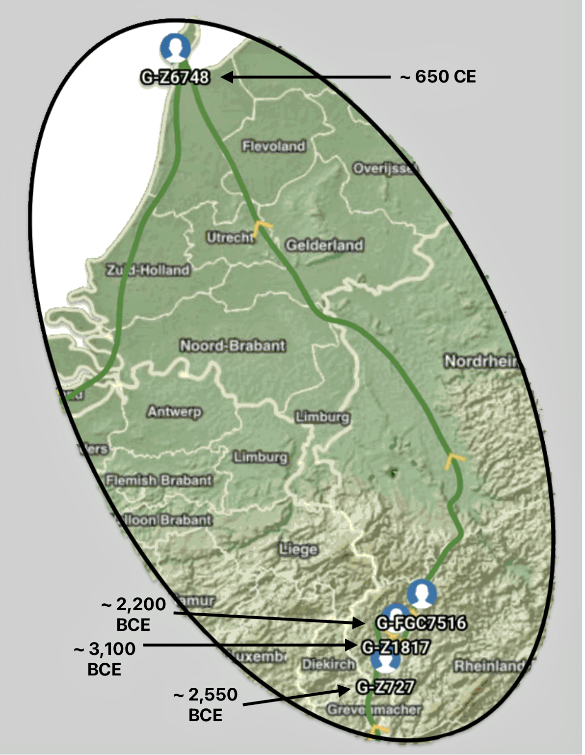
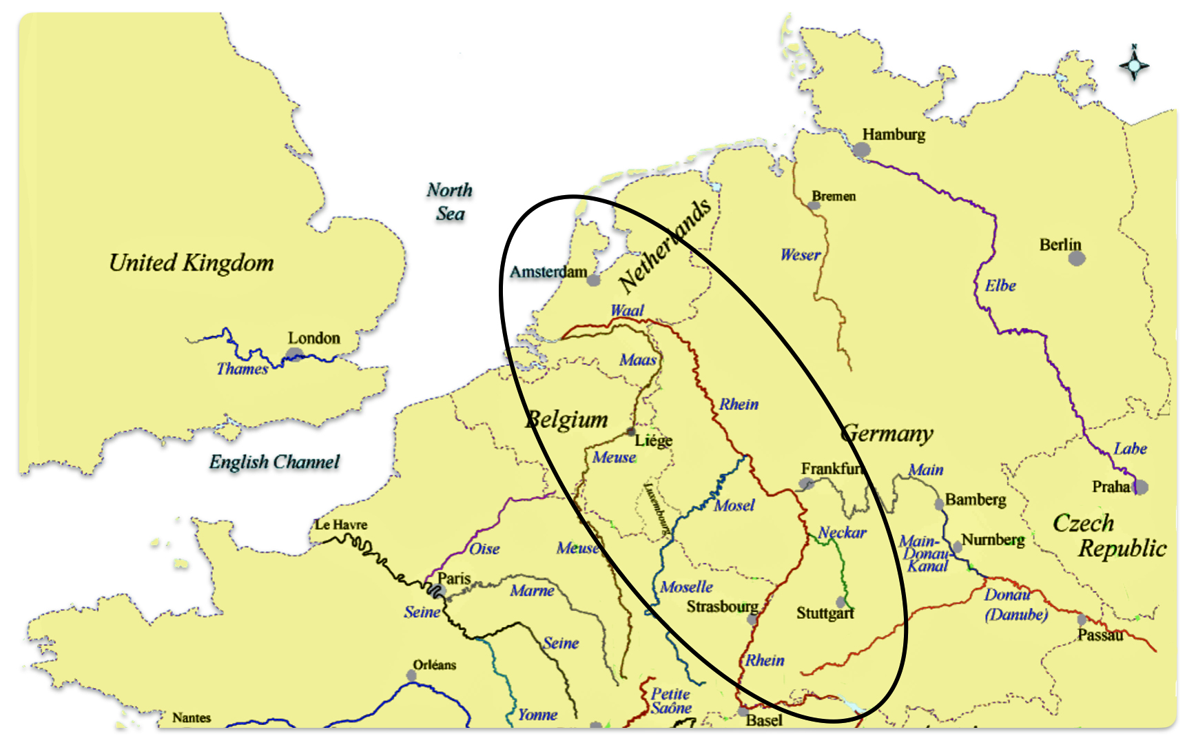
The estimated northward migratory path is in an area that has many rivers that may have influenced and facilitated migratory travel, as depicted in illustration ten. There are a number of major tributaries around the estimated migratory path of the Griff(is)(es)(ith paternal YDNA line: the Rhine, the Meuse, the Maas, the Waal, the Mosel, and the Neckar rivers.
Illustration Ten: Rivers in Northwestern Europe
The cultural landscape of northwestern Europe underwent dramatic transformations between 2200 BCE and 650 CE, spanning the transition from the Late Neolithic through the Bronze Age, Iron Age, Roman period, and into the early Medieval era. This period witnessed significant shifts in technology, social organization, settlement patterns, and ethnic composition, driven by a complex interplay of migration, trade, technological innovation, and political developments.
Part Two of this Story
There are a number of possible explanations for these phylogenetic gaps that are uniquely tied to demographic, social and historic influences in each of these time periods. There also are obvious methodogical explanations for each of the two historical historical gaps in phylogenetic branching. The second part of this story discusses possible explanations and the social and cultural influences in these time periods associated with the two phylogenetic gaps.
Source:
Feature Banner: The banner at the top of the story is a modification of a shapshot taken from the FamilyTreeDNA GlobetrekkerTM video of the migratory path of my YDNA descendants over time. The map shows the maigratory path of selected most common recent ancestors and their respective eestimated dates of birth. In addition the map highlights two time periods where there was a signficant time period inbetween haplogroups that are discussed in the present story.
[1] Brandt G, Haak W, Adler CJ, Roth C, Szécsényi-Nagy A, Karimnia S, Möller-Rieker S, Meller H, Ganslmeier R, Friederich S, Dresely V, Nicklisch N, Pickrell JK, Sirocko F, Reich D, Cooper A, Alt KW; Genographic Consortium. Ancient DNA reveals key stages in the formation of central European mitochondrial genetic diversity. Science. 2013 Oct 11;342(6155):257-61. doi: 10.1126/science.1241844. PMID: 24115443; PMCID: PMC4039305, (PubMed) https://pmc.ncbi.nlm.nih.gov/articles/PMC4039305/
Brotherton, P., Haak, W., Templeton, J. et al. Neolithic mitochondrial haplogroup H genomes and the genetic origins of Europeans. Nat Commun 4, 1764 (2013). https://doi.org/10.1038/ncomms2656
Early European Farmers, Wikipedia, This page was last edited on 9 March 2025, https://en.wikipedia.org/wiki/Early_European_Farmers
[2] Brandt G, Haak W, Adler CJ, Roth C, Szécsényi-Nagy A, Karimnia S, Möller-Rieker S, Meller H, Ganslmeier R, Friederich S, Dresely V, Nicklisch N, Pickrell JK, Sirocko F, Reich D, Cooper A, Alt KW; Genographic Consortium. Ancient DNA reveals key stages in the formation of central European mitochondrial genetic diversity. Science. 2013 Oct 11;342(6155):257-61. doi: 10.1126/science.1241844. PMID: 24115443; PMCID: PMC4039305, (PubMed) https://pmc.ncbi.nlm.nih.gov/articles/PMC4039305/
Hervella M, Izagirre N, Alonso S, Fregel R, Alonso A, Cabrera VM, de la Rúa C. Ancient DNA from hunter-gatherer and farmer groups from Northern Spain supports a random dispersion model for the Neolithic expansion into Europe. PLoS One. 2012;7(4):e34417. doi: 10.1371/journal.pone.0034417. Epub 2012 Apr 25. Erratum in: PLoS One. 2012;7(7). doi:10.1371/annotation/3dac0b4f-f76e-4bc1-8559-acb41b87b02c. PMID: 22563371; PMCID: PMC3340892, (PubMed) https://pmc.ncbi.nlm.nih.gov/articles/PMC3340892/
Posth, C., Yu, H., Ghalichi, A. et al. Palaeogenomics of Upper Palaeolithic to Neolithic European hunter-gatherers. Nature 615, 117–126 (2023). https://doi.org/10.1038/s41586-023-05726-0
L.G. Simões, R. Peyroteo-Stjerna, G. Marchand, C. Bernhardsson, A. Vialet, D. Chetty, E. Alaçamlı, H. Edlund, D. Bouquin, C. Dina, N. Garmond, T. Günther, & M. Jakobsson, Genomic ancestry and social dynamics of the last hunter-gatherers of Atlantic France, Proc. Natl. Acad. Sci. U.S.A. 121 (10) e2310545121, https://doi.org/10.1073/pnas.2310545121 (2024).
[3] Posth, C., Yu, H., Ghalichi, A. et al. Palaeogenomics of Upper Palaeolithic to Neolithic European hunter-gatherers. Nature 615, 117–126 (2023). https://doi.org/10.1038/s41586-023-05726-0
Maïté Rivollat et al. ,Ancient genome-wide DNA from France highlights the complexity of interactions between Mesolithic hunter-gatherers and Neolithic farmers.Sci. Adv.6,eaaz5344(2020).DOI:10.1126/sciadv.aaz5344
L.G. Simões, R. Peyroteo-Stjerna, G. Marchand, C. Bernhardsson, A. Vialet, D. Chetty, E. Alaçamlı, H. Edlund, D. Bouquin, C. Dina, N. Garmond, T. Günther, & M. Jakobsson, Genomic ancestry and social dynamics of the last hunter-gatherers of Atlantic France, Proc. Natl. Acad. Sci. U.S.A. 121 (10) e2310545121, https://doi.org/10.1073/pnas.2310545121 (2024).
[4] Western Steppe Herders, Wikipedia, This page was last edited on 27 March 2025, https://en.wikipedia.org/wiki/Western_Steppe_Herders
Haak W, Lazaridis I, Patterson N, Rohland N, Mallick S, Llamas B, Brandt G, Nordenfelt S, Harney E, Stewardson K, Fu Q, Mittnik A, Bánffy E, Economou C, Francken M, Friederich S, Pena RG, Hallgren F, Khartanovich V, Khokhlov A, Kunst M, Kuznetsov P, Meller H, Mochalov O, Moiseyev V, Nicklisch N, Pichler SL, Risch R, Rojo Guerra MA, Roth C, Szécsényi-Nagy A, Wahl J, Meyer M, Krause J, Brown D, Anthony D, Cooper A, Alt KW, Reich D. Massive migration from the steppe was a source for Indo-European languages in Europe. Nature. 2015 Jun 11;522(7555):207-11. doi: 10.1038/nature14317. Epub 2015 Mar 2. PMID: 25731166; PMCID: PMC5048219, (PubMed) https://pmc.ncbi.nlm.nih.gov/articles/PMC5048219/, see also https://reich.hms.harvard.edu/sites/reich.hms.harvard.edu/files/inline-files/nature14317.pdf
[5] Brandt G, et al , Ancient DNA reveals key stages in the formation of central European mitochondrial genetic diversity. Science. 2013 Oct 11;342(6155):257-61. doi: 10.1126/science.1241844. PMID: 24115443; PMCID: PMC4039305, (PubMed) https://pmc.ncbi.nlm.nih.gov/articles/PMC4039305/
Z. Hofmanová, S. Kreutzer, G. Hellenthal, C. Sell, et al , Early farmers from across Europe directly descended from Neolithic Aegeans, Proc. Natl. Acad. Sci. U.S.A.113 (25) 6886-6891, https://doi.org/10.1073/pnas.1523951113 (2016).
Fernández E, Pérez-Pérez A, Gamba C, Prats E, Cuesta P, Anfruns J, Molist M, Arroyo-Pardo E, Turbón D. Ancient DNA analysis of 8000 B.C. near eastern farmers supports an early neolithic pioneer maritime colonization of Mainland Europe through Cyprus and the Aegean Islands. PLoS Genet. 2014 Jun 5;10(6):e1004401. doi: 10.1371/journal.pgen.1004401. PMID: 24901650; PMCID: PMC4046922, (PubMed) https://pmc.ncbi.nlm.nih.gov/articles/PMC4046922/
[6] Brandt G, et al ,Ancient DNA reveals key stages in the formation of central European mitochondrial genetic diversity. Science. 2013 Oct 11;342(6155):257-61. doi: 10.1126/science.1241844. PMID: 24115443; PMCID: PMC4039305, (PubMed) https://pmc.ncbi.nlm.nih.gov/articles/PMC4039305/
Hervella M, Izagirre N, Alonso S, Fregel R, Alonso A, Cabrera VM, de la Rúa C. Ancient DNA from hunter-gatherer and farmer groups from Northern Spain supports a random dispersion model for the Neolithic expansion into Europe. PLoS One. 2012;7(4):e34417. doi: 10.1371/journal.pone.0034417. Epub 2012 Apr 25. Erratum in: PLoS One. 2012;7(7). doi:10.1371/annotation/3dac0b4f-f76e-4bc1-8559-acb41b87b02c. PMID: 22563371; PMCID: PMC3340892, (PubMed) https://pmc.ncbi.nlm.nih.gov/articles/PMC3340892/
Brotherton, P., Haak, W., Templeton, J. et al. Neolithic mitochondrial haplogroup H genomes and the genetic origins of Europeans. Nat Commun 4, 1764 (2013). https://doi.org/10.1038/ncomms2656
[7] Brotherton, P., Haak, W., Templeton, J. et al. Neolithic mitochondrial haplogroup H genomes and the genetic origins of Europeans. Nat Commun 4, 1764 (2013). https://doi.org/10.1038/ncomms2656
Maïté Rivollat et al. Ancient genome-wide DNA from France highlights the complexity of interactions between Mesolithic hunter-gatherers and Neolithic farmers.Sci. Adv.6,eaaz5344(2020).DOI:10.1126/sciadv.aaz5344
Early European Farmers, Wikipedia, This page was last edited on 9 March 2025, https://en.wikipedia.org/wiki/Early_European_Farmers
[8] Szécsényi-Nagy A, Brandt G, Haak W, Keerl V, Jakucs J, Möller-Rieker S, Köhler K, Mende BG, Oross K, Marton T, Osztás A, Kiss V, Fecher M, Pálfi G, Molnár E, Sebők K, Czene A, Paluch T, Šlaus M, Novak M, Pećina-Šlaus N, Ősz B, Voicsek V, Somogyi K, Tóth G, Kromer B, Bánffy E, Alt KW. Tracing the genetic origin of Europe’s first farmers reveals insights into their social organization. Proc Biol Sci. 2015 Apr 22;282(1805):20150339. doi: 10.1098/rspb.2015.0339. PMID: 25808890; PMCID: PMC4389623, https://pmc.ncbi.nlm.nih.gov/articles/PMC4389623/
Fort, J., Pérez-Losada, J. Interbreeding between farmers and hunter-gatherers along the inland and Mediterranean routes of Neolithic spread in Europe. Nat Commun 15, 7032 (2024). https://doi.org/10.1038/s41467-024-51335-4
Ainash Childebayeva, Adam Benjamin Rohrlach, Rodrigo Barquera, Maïté Rivollat, Franziska Aron, András Szolek, Oliver Kohlbacher, Nicole Nicklisch, Kurt W. Alt, Detlef Gronenborn, Harald Meller, Susanne Friederich, Kay Prüfer, Marie-France Deguilloux, Johannes Krause, Wolfgang Haak, Population Genetics and Signatures of Selection in Early Neolithic European Farmers, Molecular Biology and Evolution, Volume 39, Issue 6, June 2022, msac108, https://doi.org/10.1093/molbev/msac108
[9] Szécsényi-Nagy A, et. al., Tracing the genetic origin of Europe’s first farmers reveals insights into their social organization. Proc Biol Sci. 2015 Apr 22;282(1805):20150339. doi: 10.1098/rspb.2015.0339. PMID: 25808890; PMCID: PMC4389623, https://pmc.ncbi.nlm.nih.gov/articles/PMC4389623/
Ainash Childebayeva, et al., Population Genetics and Signatures of Selection in Early Neolithic European Farmers, Molecular Biology and Evolution, Volume 39, Issue 6, June 2022, msac108, https://doi.org/10.1093/molbev/msac108
[10] Brandt G, et al ,Ancient DNA reveals key stages in the formation of central European mitochondrial genetic diversity. Science. 2013 Oct 11;342(6155):257-61. doi: 10.1126/science.1241844. PMID: 24115443; PMCID: PMC4039305, (PubMed) https://pmc.ncbi.nlm.nih.gov/articles/PMC4039305/
Juras, A., Chyleński, M., Ehler, E. et al. Mitochondrial genomes reveal an east to west cline of steppe ancestry in Corded Ware populations. Sci Rep 8, 11603 (2018). https://doi.org/10.1038/s41598-018-29914-5
Maja Krzewińska et al. ,Ancient genomes suggest the eastern Pontic-Caspian steppe as the source of western Iron Age nomads.Sci. Adv.4,eaat4457(2018).DOI:10.1126/sciadv.aat4457 , https://www.science.org/doi/10.1126/sciadv.aat4457
[11] Juras, A., Chyleński, M., Ehler, E. et al. Mitochondrial genomes reveal an east to west cline of steppe ancestry in Corded Ware populations. Sci Rep 8, 11603 (2018). https://doi.org/10.1038/s41598-018-29914-5
Wolfgang Haak, Iosif Lazaridis, Nick Patterson, Nadin Rohland, Swapan Mallic, Bastien Llamas1, Guido Brandt, et al, Massive migration from the steppe was a source for Indo-European languages in Europe, Research Letter, 2015, Nature, https://reich.hms.harvard.edu/sites/reich.hms.harvard.edu/files/inline-files/nature14317.pdf
[12] Brandt G, et al ,Ancient DNA reveals key stages in the formation of central European mitochondrial genetic diversity. Science. 2013 Oct 11;342(6155):257-61. doi: 10.1126/science.1241844. PMID: 24115443; PMCID: PMC4039305, (PubMed) https://pmc.ncbi.nlm.nih.gov/articles/PMC4039305/
Brotherton, P., Haak, W., Templeton, J. et al. Neolithic mitochondrial haplogroup H genomes and the genetic origins of Europeans. Nat Commun 4, 1764 (2013). https://doi.org/10.1038/ncomms2656
Early European Farmers, Wikipedia, This page was last edited on 9 March 2025, https://en.wikipedia.org/wiki/Early_European_Farmers
[13] Western Steppe Herders, Wikipedia, This page was last edited on 27 March 2025, https://en.wikipedia.org/wiki/Western_Steppe_Herders
Haak W, Lazaridis I, Patterson N, Rohland N, Mallick S, Llamas B, Brandt G, Nordenfelt S, Harney E, Stewardson K, Fu Q, Mittnik A, Bánffy E, Economou C, Francken M, Friederich S, Pena RG, Hallgren F, Khartanovich V, Khokhlov A, Kunst M, Kuznetsov P, Meller H, Mochalov O, Moiseyev V, Nicklisch N, Pichler SL, Risch R, Rojo Guerra MA, Roth C, Szécsényi-Nagy A, Wahl J, Meyer M, Krause J, Brown D, Anthony D, Cooper A, Alt KW, Reich D. Massive migration from the steppe was a source for Indo-European languages in Europe. Nature. 2015 Jun 11;522(7555):207-11. doi: 10.1038/nature14317. Epub 2015 Mar 2. PMID: 25731166; PMCID: PMC5048219, (Pubmed) https://pmc.ncbi.nlm.nih.gov/articles/PMC5048219/
Wolfgang Haak, Iosif Lazaridis, Nick Patterson, Nadin Rohland, Swapan Mallic, Bastien Llamas1, Guido Brandt, et al, Massive migration from the steppe was a source for Indo-European languages in Europe, Research Letter, 2015, Nature, https://reich.hms.harvard.edu/sites/reich.hms.harvard.edu/files/inline-files/nature14317.pdf
[14] Wolfgang Haak, Iosif Lazaridis, Nick Patterson, Nadin Rohland, Swapan Mallic, Bastien Llamas1, Guido Brandt, et al, Massive migration from the steppe was a source for Indo-European languages in Europe, Research Letter, 2015, Nature, https://reich.hms.harvard.edu/sites/reich.hms.harvard.edu/files/inline-files/nature14317.pdf
Haak W, Lazaridis I, Patterson N, Rohland N, et al , Massive migration from the steppe was a source for Indo-European languages in Europe. Nature. 2015 Jun 11;522(7555):207-11. doi: 10.1038/nature14317. Epub 2015 Mar 2. PMID: 25731166; PMCID: PMC5048219, (Pubmed) https://pmc.ncbi.nlm.nih.gov/articles/PMC5048219/
Juras, A., Chyleński, M., Ehler, E. et al. Mitochondrial genomes reveal an east to west cline of steppe ancestry in Corded Ware populations. Sci Rep 8, 11603 (2018). https://doi.org/10.1038/s41598-018-29914-5
[15] Wolfgang Haak, Iosif Lazaridis, Nick Patterson, Nadin Rohland, Swapan Mallic, Bastien Llamas1, Guido Brandt, et al, Massive migration from the steppe was a source for Indo-European languages in Europe, Research Letter, 2015, Nature, https://reich.hms.harvard.edu/sites/reich.hms.harvard.edu/files/inline-files/nature14317.pdf
Haak W, Lazaridis I, Patterson N, Rohland N, et al , Massive migration from the steppe was a source for Indo-European languages in Europe. Nature. 2015 Jun 11;522(7555):207-11. doi: 10.1038/nature14317. Epub 2015 Mar 2. PMID: 25731166; PMCID: PMC5048219, (Pubmed) https://pmc.ncbi.nlm.nih.gov/articles/PMC5048219/
[16] Mittnik, A., Wang, CC., Pfrengle, S. et al. The genetic prehistory of the Baltic Sea region.Nat Commun 9, 442 (2018). https://doi.org/10.1038/s41467-018-02825-9
[17] Brotherton, P., Haak, W., Templeton, J. et al. Neolithic mitochondrial haplogroup H genomes and the genetic origins of Europeans. Nat Commun 4, 1764 (2013). https://doi.org/10.1038/ncomms2656
Daniel M. Fernandes, Alissa Mittnik, et al, The spread of steppe and Iranian-related ancestry in the islands of the western Mediterranean, Nature Ecology & Evolution, https://reich.hms.harvard.edu/sites/reich.hms.harvard.edu/files/inline-files/2020_Fernandes_NatEcolEvol_WestMediterranean_0.pdf
[18] Early European Farmers, Wikipedia, This page was last edited on 9 March 2025, https://en.wikipedia.org/wiki/Early_European_Farmers
Narva, Wikipedia, This page was last edited on 7 April 2025, https://en.wikipedia.org/wiki/Narva
[19] Brotherton, P., Haak, W., Templeton, J. et al. Neolithic mitochondrial haplogroup H genomes and the genetic origins of Europeans. Nat Commun 4, 1764 (2013). https://doi.org/10.1038/ncomms2656
Daniel M. Fernandes, Alissa Mittnik, Iñigo Olalde, et al., The spread of steppe and Iranian-related ancestry in the islands of the western Mediterranean, Nature Ecology & Evolution , https://doi.org/10.1038/s41559-020-1102-0 , https://reich.hms.harvard.edu/sites/reich.hms.harvard.edu/files/inline-files/2020_Fernandes_NatEcolEvol_WestMediterranean_0.pdf
[20] Early European Farmers, Wikipedia, This page was last edited on 9 March 2025, https://en.wikipedia.org/wiki/Early_European_Farmers
[21] Sjur Cappelen Papazian, The spread of haplogroup G2a in Europe, 2 Nov 2013, Cradle of Civilization, https://aratta.wordpress.com/2013/11/02/bell-beakers/
Hay, Maciamo, Distribution of G2a in Italy (Boattini et al.), 7 jun 2013, Forum, Eupedia, https://www.eupedia.com/forum/threads/distribution-of-g2a-in-italy-boattini-et-al.28663/
Hay, Maciamo, Origins and history of Haplogroup G2a (Y-DNA), Oct 2016, https://www.academia.edu/6173684/Origins_and_history_of_Haplogroup_G2a_Y_DNA_
Hay, Maciamo, Haplogroup G2a (Y-DNA), July 2023, Eupedia, https://www.eupedia.com/europe/Haplogroup_G2a_Y-DNA.shtml
[22] Laura Spinney’s article “When the First Farmers Arrived in Europe, Inequality Evolved” highlights several key points regarding the societal changes and the rise of inequality associated with the arrival of agriculture in Europe.
Long-term Impacts on European Society: The establishment of farming led to surplus food production, which facilitated trade and storage but also created conditions for social stratification and inequality. Communities became more complex socially and economically, laying foundations for later societal structures characterized by hierarchy and unequal resource distribution
Introduction of Agriculture and Inequality: The arrival of the first farmers in Europe, migrating from Anatolia around 7,000 BC, marked a significant shift from hunter-gatherer societies to settled agricultural communities. This transition led to increased population densities and sedentary lifestyles.
Emergence of Social Hierarchies: With agriculture came surplus food production, which allowed for accumulation of resources. This surplus facilitated the development of social hierarchies and economic disparities, as some individuals or groups could accumulate more resources than others, leading to the evolution of inequality.
Genetic Evidence of Social Stratification: Archaeogenetic studies revealed that early European farmers initially mixed minimally with local hunter-gatherers; however, during the Middle Neolithic period, there was increased mixing predominantly involving hunter-gatherer males and farmer females. This pattern suggests a social structure where hunter-gatherer men integrated into farming communities, potentially reflecting power dynamics or social stratification.
Violence and Competition: The archaeological record includes evidence of violence among early farming groups, such as the systematic massacre at Els Trocs in Spain, indicating competition for resources or territory among early agricultural communities.
Spinney, Laura, When the First Farmers Arrived in Europe, Inequality Evolved, 1 Jul 2020, Scientific American, https://www.scientificamerican.com/article/when-the-first-farmers-arrived-in-europe-inequality-evolved/
See also:
The genetic origins of the world’s first farmers clarified, 2022, Univerität Bern, https://mediarelations.unibe.ch/media_releases/2022/media_releases_2022/the_genetic_origins_of_the_worlds_first_farmers_clarified/index_eng.html
The genetic origins of the world’s first farmers clarified, 12 May 2022, EurekAlert!, University of Bern, https://www.eurekalert.org/news-releases/952510
Marchi, Winkelbach, Schulz, Brami et al., The genomic origins of the world’s first farmers, Cell (2022), doi: 10.1016/j.cell.2022.04.00, https://www.cell.com/cell/fulltext/S0092-8674(22)00455-X
Ainash Childebayeva, Adam Benjamin Rohrlach, Rodrigo Barquera, Maïté Rivollat, Franziska Aron, András Szolek, Oliver Kohlbacher, Nicole Nicklisch, Kurt W. Alt, Detlef Gronenborn, Harald Meller, Susanne Friederich, Kay Prüfer, Marie-France Deguilloux, Johannes Krause, Wolfgang Haak, Population Genetics and Signatures of Selection in Early Neolithic European Farmers, Molecular Biology and Evolution, Volume 39, Issue 6, June 2022, msac108, https://doi.org/10.1093/molbev/msac108
Szécsényi-Nagy A, Brandt G, Haak W, Keerl V, Jakucs J, Möller-Rieker S, Köhler K, Mende BG, Oross K, Marton T, Osztás A, Kiss V, Fecher M, Pálfi G, Molnár E, Sebők K, Czene A, Paluch T, Šlaus M, Novak M, Pećina-Šlaus N, Ősz B, Voicsek V, Somogyi K, Tóth G, Kromer B, Bánffy E, Alt KW. Tracing the genetic origin of Europe’s first farmers reveals insights into their social organization. Proc Biol Sci. 2015 Apr 22;282(1805):20150339. doi: 10.1098/rspb.2015.0339. PMID: 25808890; PMCID: PMC4389623, https://pmc.ncbi.nlm.nih.gov/articles/PMC4389623/
Isern, N., Fort, J. & de Rioja, V.L. The ancient cline of haplogroup K implies that the Neolithic transition in Europe was mainly demic. Sci Rep 7, 11229 (2017). https://doi.org/10.1038/s41598-017-11629-8
Reich, David (2018). Who We are and how We Got Here: Ancient DNA and the New Science of the Human Past. Oxford University Press.
Early European Farmers, Wikipedia, This page was last edited on 8 December 2024, https://en.wikipedia.org/wiki/Early_European_Farmers
Lazaridis, Iosif; et al. (25 July 2016). “Genomic insights into the origin of farming in the ancient Near East”. Nature. 536 (7617). Nature Research: 419–424. Bibcode:2016Natur.536..419L. doi:10.1038/nature19310
Lazaridis, Losif , “The evolutionary history of human populations in Europe”, Dec 2018, Current Opinion in Genetics & Development. 53, Elsevier: 21–27. arXiv:1805.01579. doi:10.1016/j.gde.2018.06.007
Shennan, Stephen (2018). The First Farmers of Europe: An Evolutionary Perspective. Cambridge World Archaeology. Cambridge University Press. doi:10.1017/9781108386029
[23] The Middle Neolithic era, a period within the broader Neolithic period, is characterized by the flourishing of settled agricultural communities, the development of new technologies, and the emergence of distinct regional cultures, roughly spanning from around 3300 to 2900 BCE in some regions.
The Middle Neolithic saw a continuation and intensification of settled agricultural practices, with communities relying on domesticated plants and animals for sustenance. This period saw the development and refinement of tools, pottery, and other technologies, including the use of polished stone tools and the emergence of new forms of pottery. The Middle Neolithic period saw the development of distinct regional cultures, with variations in material culture, settlement patterns, and social organization. The increased sedentism and agricultural surplus led to the development of more complex social structures, with evidence of social stratification and specialization of labor.
A prominent Middle Neolithic culture in Central Europe, the Linear Pottery Culture (LBK) was known for its distinctive pottery and settlement pattern.
Fay Worley, Richard Madgwick, Ruth Pelling, Peter Marshall, Jane A. Evans, Angela L. Lamb, Inés L. López-Dóriga, Christopher Bronk Ramsey, Elaine Dunbar, Paula Reimer, John Vallender, David Roberts, Understanding Middle Neolithic food and farming in and around the Stonehenge World Heritage Site: An integrated approach, Journal of Archaeological Science: Reports, Volume 26, 2019, 101838, ISSN 2352-409X, https://doi.org/10.1016/j.jasrep.2019.05.003 .
(https://www.sciencedirect.com/science/article/pii/S2352409X18307892 )
Neolithic Revolution, Wikipeida, This page was last edited on 25 March 2025, https://en.wikipedia.org/wiki/Neolithic_Revolution
Neolitchic Europe, Wikipedia, This page was last edited on 20 March 2025, https://en.wikipedia.org/wiki/Neolithic_Europe
[24] Hervella M, Izagirre N, Alonso S, Fregel R, Alonso A, Cabrera VM, de la Rúa C. Ancient DNA from hunter-gatherer and farmer groups from Northern Spain supports a random dispersion model for the Neolithic expansion into Europe. PLoS One. 2012;7(4):e34417. doi: 10.1371/journal.pone.0034417. Epub 2012 Apr 25. Erratum in: PLoS One. 2012;7(7). doi:10.1371/annotation/3dac0b4f-f76e-4bc1-8559-acb41b87b02c. PMID: 22563371; PMCID: PMC3340892, (PubMed) https://pmc.ncbi.nlm.nih.gov/articles/PMC3340892/
[25] Spinney, Laura, When the First Farmers Arrived in Europe, Inequality Evolved, 1 Jul 2020, Scientific American, https://www.scientificamerican.com/article/when-the-first-farmers-arrived-in-europe-inequality-evolved/
Marchi N, Winkelbach L, Schulz I, Brami M, Hofmanová Z, Blöcher J, Reyna-Blanco CS, Diekmann Y, Thiéry A, Kapopoulou A, Link V, Piuz V, Kreutzer S, Figarska SM, Ganiatsou E, Pukaj A, Struck TJ, Gutenkunst RN, Karul N, Gerritsen F, Pechtl J, Peters J, Zeeb-Lanz A, Lenneis E, Teschler-Nicola M, Triantaphyllou S, Stefanović S, Papageorgopoulou C, Wegmann D, Burger J, Excoffier L. The genomic origins of the world’s first farmers. Cell. 2022 May 26;185(11):1842-1859.e18. doi: 10.1016/j.cell.2022.04.008. Epub 2022 May 12. PMID: 35561686; PMCID: PMC9166250, (PubMed) https://pubmed.ncbi.nlm.nih.gov/35561686/
[26] Patrilocal residence, Wikipedia, This page was last edited on 20 January 2024, https://en.wikipedia.org/wiki/Patrilocal_residence
[27] Marchi N, Winkelbach L, Schulz I, Brami M, Hofmanová Z, Blöcher J, Reyna-Blanco CS, Diekmann Y, Thiéry A, Kapopoulou A, Link V, Piuz V, Kreutzer S, Figarska SM, Ganiatsou E, Pukaj A, Struck TJ, Gutenkunst RN, Karul N, Gerritsen F, Pechtl J, Peters J, Zeeb-Lanz A, Lenneis E, Teschler-Nicola M, Triantaphyllou S, Stefanović S, Papageorgopoulou C, Wegmann D, Burger J, Excoffier L. The genomic origins of the world’s first farmers. Cell. 2022 May 26;185(11):1842-1859.e18. doi: 10.1016/j.cell.2022.04.008. Epub 2022 May 12. PMID: 35561686; PMCID: PMC9166250, (PubMed) https://pmc.ncbi.nlm.nih.gov/articles/PMC9166250/
The genetic origins of the world’s first farmers clarified, 12 May 2022, New Release, University of Bern, https://www.eurekalert.org/news-releases/952510
[28] Jordans, Frank, Study: Aegean farmers replaced hunters of ancient Britain, 15 April 2019, Phys.Org, https://phys.org/news/2019-04-aegean-farmers-hunters-ancient-britain.html
Brace, S., Diekmann, Y., Booth, T.J. et al. Ancient genomes indicate population replacement in Early Neolithic Britain. Nat Ecol Evol 3, 765–771 (2019). https://doi.org/10.1038/s41559-019-0871-9
[29] Eppie R. Jones, Gunita Zarina, Vyacheslav Moiseyev, Emma Lightfoot, Philip R. Nigst, Andrea Manica, Ron Pinhasi, and Daniel G. Bradley, The Neolithic Transition in the Baltic Was Not Driven by Admixture with Early European Farmers, Current Biology 27, 576–582, February 20, 2017, 576-582, https://www.cell.com/current-biology/fulltext/S0960-9822(16)31542-1
[30] Gloria González-Fortes, Eppie R. Jones, Emma Lightfoot, Clive Bonsall, Catalin Lazar, Aurora Grandal-d’Anglade, María Dolores Garralda, Labib Drak, Veronika Siska, Angela Simalcsik, Adina Boroneanţ, Juan Ramón Vidal Romaní, Marcos Vaqueiro Rodríguez, Pablo Arias, Ron Pinhasi, Andrea Manica, Michael Hofreiter, Paleogenomic Evidence for Multi-generational Mixing between Neolithic Farmers and Mesolithic Hunter-Gatherers in the Lower Danube Basin, Current Biology, Volume 27, Issue 12, 2017, Pages 1801-1810.e10, ISSN 0960-9822,
https://doi.org/10.1016/j.cub.2017.05.023 .
(https://www.sciencedirect.com/science/article/pii/S0960982217305596 )
[31] Fort J, Pérez-Losada J. Interbreeding between farmers and hunter-gatherers along the inland and Mediterranean routes of Neolithic spread in Europe. Nat Commun. 2024 Aug 15;15(1):7032. doi: 10.1038/s41467-024-51335-4. PMID: 39147743; PMCID: PMC11327347, (PubMed) https://pubmed.ncbi.nlm.nih.gov/39147743/
[32] Alexandros Tsoupas, Carlos S. Reyna-Blanco, Claudio S. Quilodrán, Jens Blöcher, Maxime Brami, Daniel Wegmann, Joachim Burger, Mathias Currat, Local increases in admixture with hunter-gatherers followed the initial expansion of Neolithic farmers across continental Europe, bioRxiv, June 12, 2024,. 598301; doi: https://doi.org/10.1101/2024.06.10.598301
[33] Maïté Rivollat et al. ,Ancient genome-wide DNA from France highlights the complexity of interactions between Mesolithic hunter-gatherers and Neolithic farmers.Sci. Adv.6,eaaz5344(2020).DOI:10.1126/sciadv.aaz5344
[34] Peter Rowley-Conwy, Westward Ho! The Spread of Agriculture from Central Europe to the Atlantic, Current Anthropology Volume 52, Supplement 4, October 2011, S431-451, https://www.journals.uchicago.edu/doi/epdf/10.1086/658368
Neolithic Revolution, Wikipedia, This page was last edited on 7 April 2025, https://en.wikipedia.org/wiki/Neolithic_Revolution
[35] Spinney, Laura, When the First Farmers Arrived in Europe, Inequality Evolved, 1 Jul 2020, Scientific American, https://www.scientificamerican.com/article/when-the-first-farmers-arrived-in-europe-inequality-evolved/
[36] Bogucki, Peter and Ryszard Grygiel, Farmers of the North European Plain, Scientific American, Vol. 248, No. 4 (April 1983), pp. 104-113l https://www.jstor.org/stable/10.2307/24968879
Oelze, Vicky & Münster, Angelina & Nicklisch, Nicole & Meller, Harald & Dresely, Veit & Alt, Kurt. (2010). Early Neolithic diet and animal husbandry: Stable isotope evidence from three Linearbandkeramik (LBK) sites in Central Germany. Journal of Archaeological Science. 38. 270-279. DOI:10.1016/j.jas.2010.08.027
Szécsényi-Nagy A, et al. Tracing the genetic origin of Europe’s first farmers reveals insights into their social organization. Proc Biol Sci. 2015 Apr 22;282(1805):20150339. doi: 10.1098/rspb.2015.0339. PMID: 25808890; PMCID: PMC4389623, PubMed) https://pmc.ncbi.nlm.nih.gov/articles/PMC4389623/
Early Neolithic farmers arriving on the Baltic coast bucked trends and incorporated fish into their diets, 17 October 2023, University of York, https://phys.org/news/2023-10-early-neolithic-farmers-baltic-coast.html
Alexandros Tsoupas, Carlos S. Reyna-Blanco, Claudio S. Quilodrán1, Jens, Blöcher4, Maxime Brami, Daniel Wegmann, Joachim Burger, Mathias Currat, Local increases in admixture with hunter-gatherers followed the initial expansion of Neolithic farmers across continental Europe, 12 Jun 2024, bioRxiv , doi: https://doi.org/10.1101/2024.06.10.598301, https://www.biorxiv.org/content/10.1101/2024.06.10.598301v1.full.pdf+html
Maïté Rivollat et al. ,Ancient genome-wide DNA from France highlights the complexity of interactions between Mesolithic hunter-gatherers and Neolithic farmers.Sci. Adv.6,eaaz5344(2020).DOI:10.1126/sciadv.aaz534432c
[37] Peter Rowley-Conwy, Westward Ho! The Spread of Agriculture from Central Europe to the Atlantic, Current Anthropology Volume 52, Supplement 4, October 2011, S431-451, https://www.journals.uchicago.edu/doi/epdf/10.1086/658368
[38] Alexandros Tsoupas, et al, , Local increases in admixture with hunter-gatherers followed the initial expansion of Neolithic farmers across continental Europe, 12 Jun 2024, bioRxiv , doi: https://doi.org/10.1101/2024.06.10.598301, https://www.biorxiv.org/content/10.1101/2024.06.10.598301v1.full.pdf+html
Maïté Rivollat et al. ,Ancient genome-wide DNA from France highlights the complexity of interactions between Mesolithic hunter-gatherers and Neolithic farmers.Sci. Adv.6,eaaz5344(2020).DOI:10.1126/sciadv.aaz534432c
[39] Peter Rowley-Conwy, Westward Ho! The Spread of Agriculture from Central Europe to the Atlantic, Current Anthropology Volume 52, Supplement 4, October 2011, S431-451, https://www.journals.uchicago.edu/doi/epdf/10.1086/658368
[40] R. Bollongino, O. Nehlich, M. P. Richards, J. Orschiedt, M. G. Thomas, C. Sell, Z. Fajkošová, A. Powell, J. Burger, 2000 Years of Parallel Societies in Stone Age Central Europe. Science 342, 479–481 (2013)
[41] Szécsényi-Nagy A, Brandt G, Haak W, Keerl V, Jakucs J, Möller-Rieker S, Köhler K, Mende BG, Oross K, Marton T, Osztás A, Kiss V, Fecher M, Pálfi G, Molnár E, Sebők K, Czene A, Paluch T, Šlaus M, Novak M, Pećina-Šlaus N, Ősz B, Voicsek V, Somogyi K, Tóth G, Kromer B, Bánffy E, Alt KW. Tracing the genetic origin of Europe’s first farmers reveals insights into their social organization. Proc Biol Sci. 2015 Apr 22;282(1805):20150339. doi: 10.1098/rspb.2015.0339. PMID: 25808890; PMCID: PMC4389623, PubMed) https://pmc.ncbi.nlm.nih.gov/articles/PMC4389623/
Anna Szécsényi-Nagy, Guido Brandt, Wolfgang Haak, Victoria Keerl, János Jakucs, Sabine Möller-Rieker, Kitti Köhler, Balázs Gusztáv Mende, Krisztián Oross, Tibor Marton, Anett Osztás, Viktória Kiss, Marc Fecher, György Pálfi, Erika Molnár, et al , Tracing the genetic origin of Europe’s first farmers reveals insights into their social organization, 22 April 2015, Proceedings of the Royal Society B Biological Sciences, https://doi.org/10.1098/rspb.2015.0339
[42] Alexandros Tsoupas, Carlos S. Reyna-Blanco, Claudio S. Quilodrán1, Jens, Blöcher4, Maxime Brami, Daniel Wegmann, Joachim Burger, Mathias Currat, Local increases in admixture with hunter-gatherers followed the initial expansion of Neolithic farmers across continental Europe, 12 Jun 2024, bioRxiv , doi: https://doi.org/10.1101/2024.06.10.598301, https://www.biorxiv.org/content/10.1101/2024.06.10.598301v1.full.pdf+html
Maïté Rivollat et al. ,Ancient genome-wide DNA from France highlights the complexity of interactions between Mesolithic hunter-gatherers and Neolithic farmers.Sci. Adv.6,eaaz5344(2020).DOI:10.1126/sciadv.aaz5344
[43] Szécsényi-Nagy A, Brandt G, Haak W, Keerl V, Jakucs J, Möller-Rieker S, Köhler K, Mende BG, Oross K, Marton T, Osztás A, Kiss V, Fecher M, Pálfi G, Molnár E, Sebők K, Czene A, Paluch T, Šlaus M, Novak M, Pećina-Šlaus N, Ősz B, Voicsek V, Somogyi K, Tóth G, Kromer B, Bánffy E, Alt KW. Tracing the genetic origin of Europe’s first farmers reveals insights into their social organization. Proc Biol Sci. 2015 Apr 22;282(1805):20150339. doi: 10.1098/rspb.2015.0339. PMID: 25808890; PMCID: PMC4389623, https://pmc.ncbi.nlm.nih.gov/articles/PMC4389623/
[44] Alexandros Tsoupas, Carlos S. Reyna-Blanco, Claudio S. Quilodrán, Jens Blöcher, Maxime Brami, Daniel Wegmann, Joachim Burger, Mathias Currat, Local increases in admixture with hunter-gatherers followed the initial expansion of Neolithic farmers across continental Europe, bioRxiv, June 12, 2024,. 598301; doi: https://doi.org/10.1101/2024.06.10.598301
[45] Fort, Joaquim, Prehistoric spread rates and genetic clines, 6 Apr 2022 , Human Population Genetics and Genomics, 2022, 2(2), 0003
Aoki, Kenici, Interpreting the demic diffusion of early farming in Europe with a three-population model , 8 Oct 2024 ,Human Population Genetics and Genomics, 2024;4(4):0010 , https://doi.org/10.47248/hpgg2404040010
Michael Kempf, Solène Denis, Resource dependency and communication networks in Early Neolithic western Europe, Quaternary Environments and Humans,
Volume 2, Issue 5, 2024, 100014, ISSN 2950-2365, https://doi.org/10.1016/j.qeh.2024.100014 .
(https://www.sciencedirect.com/science/article/pii/S2950236524000124 )
Marko Porčića,Tamara Blagojević, Jugoslav Pendić,Sofija Stefanović, The timing and tempo of the Neolithic expansion across the Central Balkans in the light of the new radiocarbon evidence, Journal of Archaeological Science: Reports, Vol 33, Oct 2020, 102528, 1 – 12, https://www.sciencedirect.com/science/article/pii/S2352409X20303199
Peter Rowley-Conwy, Westward Ho! The Spread of Agriculture from Central Europe to the Atlantic, Current Anthropology Volume 52, Supplement 4, October 2011, S431-451, https://www.journals.uchicago.edu/doi/epdf/10.1086/658368; https://www.journals.uchicago.edu/doi/10.1086/658368
Neolitchic Revolution, Wikipdia, This page was last edited on 25 March 2025, https://en.wikipedia.org/wiki/Neolithic_Revolution
[46] Loess plains are regions characterized by extensive deposits of wind-blown silt called loess, often forming fertile soils, and are found globally, including in North America, China, and Europe. Loess formations are found in regions like the South Russian plains, the Danube Basin, and the German-Polish plains.
Loess Soil And Ground Fertility, World Atlas, https://www.worldatlas.com/articles/loess-soil-and-ground-fertility.html
Editors of Britannica, Loess Sedimentary Deposit, Aug 13, 2010, Britannica, Page accessed 10 Mar 2025, https://www.britannica.com/science/loess
Anna Szécsényi-Nagy, Guido Brandt, Wolfgang Haak, Victoria Keerl, János Jakucs, Sabine Möller-Rieker, Kitti Köhler, Balázs Gusztáv Mende, Krisztián Oross, Tibor Marton, Anett Osztás, Viktória Kiss, Marc Fecher, György Pálfi, Erika Molnár, et al , Tracing the genetic origin of Europe’s first farmers reveals insights into their social organization, 22 April 2015, Proceedings of the Royal Society B Biological Sciences, https://doi.org/10.1098/rspb.2015.0339
Kreuz, Angela & Marinova, Elena & Schäfer, Eva & Wiethold, Julian. (2005). A comparison of early Neolithic crop and weed assemblages from the Linearbandkeramik and the Bulgarian Neolithic cultures: Differences and similarities. Vegetation History and Archaeobotany. 14. 237-258. 10.1007/s00334-005-0080-0, https://www.researchgate.net/publication/226297202_A_comparison_of_early_Neolithic_crop_and_weed_assemblages_from_the_Linearbandkeramik_and_the_Bulgarian_Neolithic_cultures_Differences_and_similarities
[47] Anna Szécsényi-Nagy, et al , Tracing the genetic origin of Europe’s first farmers reveals insights into their social organization, 22 April 2015, Proceedings of the Royal Society B Biological Sciences, https://doi.org/10.1098/rspb.2015.0339
[48] Peter Rowley-Conwy, Westward Ho! The Spread of Agriculture from Central Europe to the Atlantic, Current Anthropology Volume 52, Supplement 4, October 2011, S431-451, https://www.journals.uchicago.edu/doi/epdf/10.1086/658368
[49] Anna Szécsényi-Nagy, et al , Tracing the genetic origin of Europe’s first farmers reveals insights into their social organization, 22 April 2015, Proceedings of the Royal Society B Biological Sciences, https://doi.org/10.1098/rspb.2015.0339
Maïté Rivollat et al. ,Ancient genome-wide DNA from France highlights the complexity of interactions between Mesolithic hunter-gatherers and Neolithic farmers.Sci. Adv.6,eaaz5344(2020).DOI:10.1126/sciadv.aaz5344
Alexandros Tsoupas, Carlos S. Reyna-Blanco, Claudio S. Quilodrán, Jens Blöcher, View ORCID ProfileMaxime Brami, Daniel Wegmann, Joachim Burger, Mathias Currat, Local increases in admixture with hunter-gatherers followed the initial expansion of Neolithic farmers across continental Europe, 12 Jun 2024, BioRxiv, doi: https://doi.org/10.1101/2024.06.10.598301 , https://www.biorxiv.org/content/10.1101/2024.06.10.598301v1
[50] Anthony, David W. ,The Horse, The Wheel and Language: How Bronze-Age Riders from the Eurasian Steppes Shaped the Modern World 2017
Anthony, David, Archaeology and Language: Why Archaeologists Care About the Indo-European Problem–in European Archaeology as Anthropology: Essays in Memory of Bernard Wailes ed by P.J. Crabtree and P. Bogucki, Philadelphia, University of Pennsylvania Press, 2017, 39-70
Vagheesh M. Narasimhan et al. ,The formation of human populations in South and Central Asia.Science365,eaat7487(2019).DOI:10.1126/science.aat7487
[51] Jeffries, Ella, Ancient DNA Sheds Light on the Origins of Indo-European Languages, 6 Feb 2025, Smithsonian, https://www.smithsonianmag.com/smart-news/ancient-dna-sheds-light-on-the-origins-of-indo-european-languages-180986012/
DeSmith, Christy, Landmark studies track source of Indo-European languages spoken by 40% of world, 5 Feb 2025, Harvard Gazette, https://news.harvard.edu/gazette/story/2025/02/landmark-studies-track-source-of-indo-european-languages-spoken-by-40-of-world/
[52] Anthony, David W. ,The Horse, The Wheel and Language: How Bronze-Age Riders from the Eurasian Steppes Shaped the Modern World, Princeton: Princeton University press, 2007
Anthony, David, Archaeology and Language: Why Archaeologists Care About the Indo-European Problem-in European Archaeology as Anthropology: Essays in Memory of Bernard Wailes ed by P.J. Crabtree and P. Bogucki, 32-72, Philadelphia: University of Pensylvaia Press, 2017
Vagheesh M. Narasimhan et al., The formation of human populations in South and Central Asia.Science365,eaat7487(2019).DOI:10.1126/science.aat7487
Nordqvist K, Heyd V. The Forgotten Child of the Wider Corded Ware Family: Russian Fatyanovo Culture in Context. Proceedings of the Prehistoric Society. 2020;86:65-93. doi: 10.1017/ppr.2020.9 https://www.cambridge.org/core/journals/proceedings-of-the-prehistoric-society/article/abs/forgotten-child-of-the-wider-corded-ware-family-russian-fatyanovo-culture-in-context/6309A60F638130BF6F7FD96135AA1B37
[53] Yamnaya Culture, Wikipedia, This page was last edited on 24 March 2025, https://en.wikipedia.org/wiki/Yamnaya_culture
[54] Shaw, Jonathan, Seeking the First Speakers of Indo-European Language, 5 Feb 2024, Harvard Magazine, https://www.harvardmagazine.com/2022/08/indo-european-languages
[55] Curry, Andrew, The First Europeans Weren’t Who Your Might Think, National Geographic Magazine, August 2019, online: https://www.nationalgeographic.com/culture/article/first-europeans-immigrants-genetic-testing-feature
[56] Gibbons, Ann, Thousands of horsemen may have swept into Bronze Age Europe, transforming the local population, 21 Feb 2017, Science Magazine, https://www.science.org/content/article/thousands-horsemen-may-have-swept-bronze-age-europe-transforming-local-population
[57] Gibbons, Ann, Thousands of horsemen may have swept into Bronze Age Europe, transforming the local population, 21 Feb 2017, Science Magazine, https://www.science.org/content/article/thousands-horsemen-may-have-swept-bronze-age-europe-transforming-local-population
[58] DeSmith, Christy, Landmark studies track source of Indo-European languages spoken by 40% of world, 5 Feb 2025, Harvard Gazette, https://news.harvard.edu/gazette/story/2025/02/landmark-studies-track-source-of-indo-european-languages-spoken-by-40-of-world/
Gibbons, Ann, Thousands of horsemen may have swept into Bronze Age Europe, transforming the local population, 21 Feb 2017, Science Magazine, https://www.science.org/content/article/thousands-horsemen-may-have-swept-bronze-age-europe-transforming-local-population
[59] A. Goldberg, T. Günther, N.A. Rosenberg, & M. Jakobsson, Ancient X chromosomes reveal contrasting sex bias in Neolithic and Bronze Age Eurasian migrations, Proc. Natl. Acad. Sci. U.S.A. 114 (10) 2657-2662, https://doi.org/10.1073/pnas.1616392114 (2017).
See also:
Balaresque, P., Bowden, G. R., Adams, S. M., Leung, H. Y., King, T. E., Rosser, Z. H., … & Jobling, M. A. (2010). A predominantly neolithic origin for European paternal lineages. PLoS biology, 8(1), e1000285.
Rasteiro R, Chikhi L. Female and male perspectives on the neolithic transition in Europe: clues from ancient and modern genetic data. PLoS One. 2013 Apr 17;8(4):e60944. doi: 10.1371/journal.pone.0060944. PMID: 23613761; PMCID: PMC3629215, (PubMed ) https://pubmed.ncbi.nlm.nih.gov/23613761/
Szécsényi-Nagy, Anna, et al. “Tracing the genetic origin of Europe’s first farmers reveals insights into their social organization.” Proceedings of the Royal Society B: Biological Sciences 282.1805 (2015): 20150339, https://royalsocietypublishing.org/doi/pdf/10.1098/rspb.2015.0339
Gimbutas, Marija. “The Indo-Europeanization of Europe: the intrusion of steppe pastoralists from south Russia and the transformation of Old Europe.” Word 44, no. 2 (1993): 205-222.
[60] Rivollat, M., Rohrlach, A.B., Ringbauer, H. et al. Extensive pedigrees reveal the social organization of a Neolithic community. Nature 620, 600–606 (2023). https://doi.org/10.1038/s41586-023-06350-8
[61] Proto-Indo-European society, Wikipedia, This page was last edited on 27 March 2025, https://en.wikipedia.org/wiki/Proto-Indo-European_society
Eurasian nomads, Wikipedia, This page was last edited on 30 March 2025, https://en.wikipedia.org/wiki/Eurasian_nomads
[62] Gibbons, Ann, Thousands of horsemen may have swept into Bronze Age Europe, transforming the local population, 21 Feb 2017, Science Magazine, https://www.science.org/content/article/thousands-horsemen-may-have-swept-bronze-age-europe-transforming-local-population
[63] Haak W, Lazaridis I, Patterson N, Rohland N, Mallick S, Llamas B, Brandt G, Nordenfelt S, Harney E, Stewardson K, Fu Q, Mittnik A, Bánffy E, Economou C, Francken M, Friederich S, Pena RG, Hallgren F, Khartanovich V, Khokhlov A, Kunst M, Kuznetsov P, Meller H, Mochalov O, Moiseyev V, Nicklisch N, Pichler SL, Risch R, Rojo Guerra MA, Roth C, Szécsényi-Nagy A, Wahl J, Meyer M, Krause J, Brown D, Anthony D, Cooper A, Alt KW, Reich D. Massive migration from the steppe was a source for Indo-European languages in Europe. Nature. 2015 Jun 11;522(7555):207-11. doi: 10.1038/nature14317. Epub 2015 Mar 2. PMID: 25731166; PMCID: PMC5048219, (PubMed) https://pmc.ncbi.nlm.nih.gov/articles/PMC5048219/, see also https://reich.hms.harvard.edu/sites/reich.hms.harvard.edu/files/inline-files/nature14317.pdf
[64] Haplogroup G-M201, Wikipedia, This page was last edited on 23 March 2025, https://en.wikipedia.org/wiki/Haplogroup_G-M201
[65] Haplogroup G-M201, Wikipedia, This page was last edited on 23 March 2025, https://en.wikipedia.org/wiki/Haplogroup_G-M201
Sims LM, Garvey D, Ballantyne J. Improved resolution haplogroup G phylogeny in the Y chromosome, revealed by a set of newly characterized SNPs. PLoS One. 2009 Jun 4;4(6):e5792. doi: 10.1371/journal.pone.0005792. PMID: 19495413; PMCID: PMC2686153, (PubMed) https://pmc.ncbi.nlm.nih.gov/articles/PMC2686153/
Rootsi, S., Myres, N., Lin, A. et al. Distinguishing the co-ancestries of haplogroup G Y-chromosomes in the populations of Europe and the Caucasus. Eur J Hum Genet 20, 1275–1282 (2012). https://doi.org/10.1038/ejhg.2012.86
Karmin M, Saag L, Vicente M, Wilson Sayres MA, Järve M, Talas UG, Rootsi S, Ilumäe AM, Mägi R, Mitt M, Pagani L, Puurand T, Faltyskova Z, Clemente F, Cardona A, Metspalu E, Sahakyan H, Yunusbayev B, Hudjashov G, DeGiorgio M, Loogväli EL, Eichstaedt C, Eelmets M, Chaubey G, Tambets K, Litvinov S, Mormina M, Xue Y, Ayub Q, Zoraqi G, Korneliussen TS, Akhatova F, Lachance J, Tishkoff S, Momynaliev K, Ricaut FX, Kusuma P, Razafindrazaka H, Pierron D, Cox MP, Sultana GN, Willerslev R, Muller C, Westaway M, Lambert D, Skaro V, Kovačevic L, Turdikulova S, Dalimova D, Khusainova R, Trofimova N, Akhmetova V, Khidiyatova I, Lichman DV, Isakova J, Pocheshkhova E, Sabitov Z, Barashkov NA, Nymadawa P, Mihailov E, Seng JW, Evseeva I, Migliano AB, Abdullah S, Andriadze G, Primorac D, Atramentova L, Utevska O, Yepiskoposyan L, Marjanovic D, Kushniarevich A, Behar DM, Gilissen C, Vissers L, Veltman JA, Balanovska E, Derenko M, Malyarchuk B, Metspalu A, Fedorova S, Eriksson A, Manica A, Mendez FL, Karafet TM, Veeramah KR, Bradman N, Hammer MF, Osipova LP, Balanovsky O, Khusnutdinova EK, Johnsen K, Remm M, Thomas MG, Tyler-Smith C, Underhill PA, Willerslev E, Nielsen R, Metspalu M, Villems R, Kivisild T. A recent bottleneck of Y chromosome diversity coincides with a global change in culture. Genome Res. 2015 Apr;25(4):459-66. doi: 10.1101/gr.186684.114. Epub 2015 Mar 13. PMID: 25770088; PMCID: PMC4381518, (PubMed) https://pmc.ncbi.nlm.nih.gov/articles/PMC4381518/
Balanovsky O, Zhabagin M, Agdzhoyan A, Chukhryaeva M, Zaporozhchenko V, Utevska O, Highnam G, Sabitov Z, Greenspan E, Dibirova K, Skhalyakho R, Kuznetsova M, Koshel S, Yusupov Y, Nymadawa P, Zhumadilov Z, Pocheshkhova E, Haber M, Zalloua PA, Yepiskoposyan L, Dybo A, Tyler-Smith C, Balanovska E. Deep phylogenetic analysis of haplogroup G1 provides estimates of SNP and STR mutation rates on the human Y-chromosome and reveals migrations of Iranic speakers. PLoS One. 2015 Apr 7;10(4):e0122968. doi: 10.1371/journal.pone.0122968. PMID: 25849548; PMCID: PMC4388827, (PubMed) https://pmc.ncbi.nlm.nih.gov/articles/PMC4388827/
Hay, Maciamo, Haplogroup G2a (Y-DNA), July 2023, Eupedia, https://www.eupedia.com/europe/Haplogroup_G2a_Y-DNA.shtml
[66] Hay, Maciamo, Haplogroup G2a (Y-DNA), July 2023, Eupedia, https://www.eupedia.com/europe/Haplogroup_G2a_Y-DNA.shtml
[67] E.K. Khusnutdinova, N.V. Ekomasova, M.A. Dzhaubermezov, L.R. Gabidullina, Z.R. Sufianova1, I.M. Khidiyatova, A.V. Kazantseva, S.S. Litvinov, A.Kh. Nurgalieva, D.S. Prokofieva, Distribution of Haplogroup G-P15 of the Y-chromosome Among Representatives of Ancient cultures and Modern Populations of Northern Eurasia, Opera Med Physiol. 2023. Vol. 10 (4), 57-72, doi: 10.24412/2500-2295-2023-4-57-72, https://operamedphys.org/system/tdf/pdf/06_DISTRIBUTION%20OF%20HAPLOGROUP%20G-P15_0.pdf?file=1&type=node&id=555&force=0
[68] Haplogroup G-P303, Wikipedia, This page was last edited on 10 December 2024, https://en.wikipedia.org/wiki/Haplogroup_G-P303
[69] Ibid
[70] Ibid
[71] The Big Y-700 test includes both STR and SNP results and provides matches for both. In addition to the STR markers included in the Y-111, it provides a minimum of 589 additional markers, giving you a total of 700 STRs, though only the first 111 are used for YDNA matching.
A Comparison of Our Y-DNA Tests, FamilyTreeDNA Help Center, https://help.familytreedna.com/hc/en-us/articles/5579319716111-A-Comparison-of-Our-Y-DNA-Tests#h_01HXD1PBPA4X6V39J3T9D5XKAN
[72] Timmers PRHJ, Wilson JF. Limited Effect of Y Chromosome Variation on Coronary Artery Disease and Mortality in UK Biobank-Brief Report. Arterioscler Thromb Vasc Biol. 2022 Sep;42(9):1198-1206. doi: 10.1161/ATVBAHA.122.317664. Epub 2022 Jul 14. PMID: 35861954; PMCID: PMC9394501, (PubMed) https://pmc.ncbi.nlm.nih.gov/articles/PMC9394501/
[73] The UK Biobank is a large-scale biomedical database and research resource based in the United Kingdom. It contains comprehensive, de-identified genetic, health, and lifestyle information, as well as biological samples from 500,000 volunteer participants aged 40–69 who were recruited between 2006 and 2010. The database is designed to support scientific research into the prevention, diagnosis, and treatment of serious illnesses such as cancer, heart disease, stroke, diabetes, and dementia. UK Biobank has collected and continues to collect extensive environmental, lifestyle, and genetic data on half a million participants.
The Biobank has data on the whole genome sequencing for all 500,000 participants, whole exome sequencing for 470,000 participants, genotyping (800,000 genome-wide variants and imputation to 90 million variants).
Bycroft, C., Freeman, C., Petkova, D. et al. The UK Biobank resource with deep phenotyping and genomic data. Nature 562, 203–209 (2018). https://doi.org/10.1038/s41586-018-0579-z
UK Biobank, Wikipedia, This page was last edited on 2 April 2025, https://en.wikipedia.org/wiki/UK_Biobank
About Our Data, BioBank, https://www.ukbiobank.ac.uk/enable-your-research/about-our-data
Timmers, Paul R.H.J and James F. Wilson, Limited Effect of Y Chromosome Variation on Coronary Artery Disease and Mortality in UK Biobank—Brief Report, 14 Jul 2022, Arteriosclerosis, Thrombosis and Vascular Biology, 42(9) https://doi.org/10.1161/ATVBAHA.122.317664
Timmers, Paul RHJ; Wilson, James F. (2022). Prevalence of Y chromosome haplogroups by area of birth in UK Biobank, 6 Jun 2022, University of Edinburgh. https://doi.org/10.7488/ds/3472
[74] Haplogroup G-M201, Wikipedia, This page was last edited on 23 March 2025, https://en.wikipedia.org/wiki/Haplogroup_G-M201
[75] Berger B, Niederstätter H, Erhart D, Gassner C, Schennach H, Parson W. Reprint of: high resolution mapping of Y haplogroup G in Tyrol (Austria). Forensic Sci Int Genet. 2013 Dec;7(6):624-631. doi: 10.1016/j.fsigen.2013.09.006. Epub 2013 Sep 27. Erratum in: Forensic Sci Int Genet. 2014 Mar;9:191. PMID: 24099688, (Pubmed) https://pubmed.ncbi.nlm.nih.gov/24099688/
[76] Hay, Maciamo, Haplogroup G2a (Y-DNA), July 2023, Eupedia, https://www.eupedia.com/europe/Haplogroup_G2a_Y-DNA.shtml
Rootsi, S., Myres, N., Lin, A. et al. Distinguishing the co-ancestries of haplogroup G Y-chromosomes in the populations of Europe and the Caucasus. Eur J Hum Genet 20, 1275–1282 (2012). https://doi.org/10.1038/ejhg.2012.86
[77] Haplogroup G-P303, Wikipedia, This page was last edited on 10 December 2024, https://en.wikipedia.org/wiki/Haplogroup_G-P303
[78] Berger B, Niederstätter H, Erhart D, Gassner C, Schennach H, Parson W. High resolution mapping of Y haplogroup G in Tyrol (Austria). Forensic Sci Int Genet. 2013 Sep;7(5):529-36. doi: 10.1016/j.fsigen.2013.05.013. Epub 2013 Jul 2. PMID: 23948323. (PubMed) https://pubmed.ncbi.nlm.nih.gov/23948323/
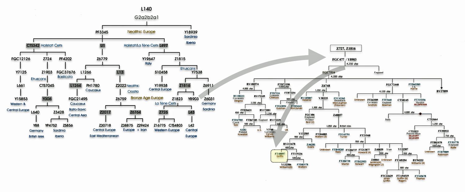
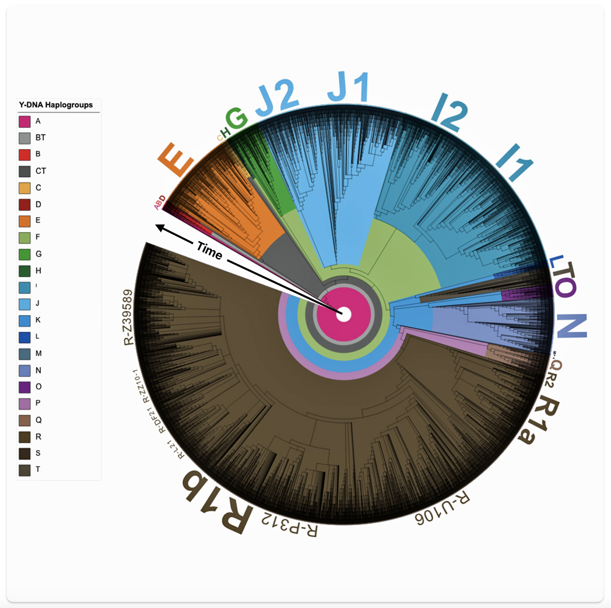
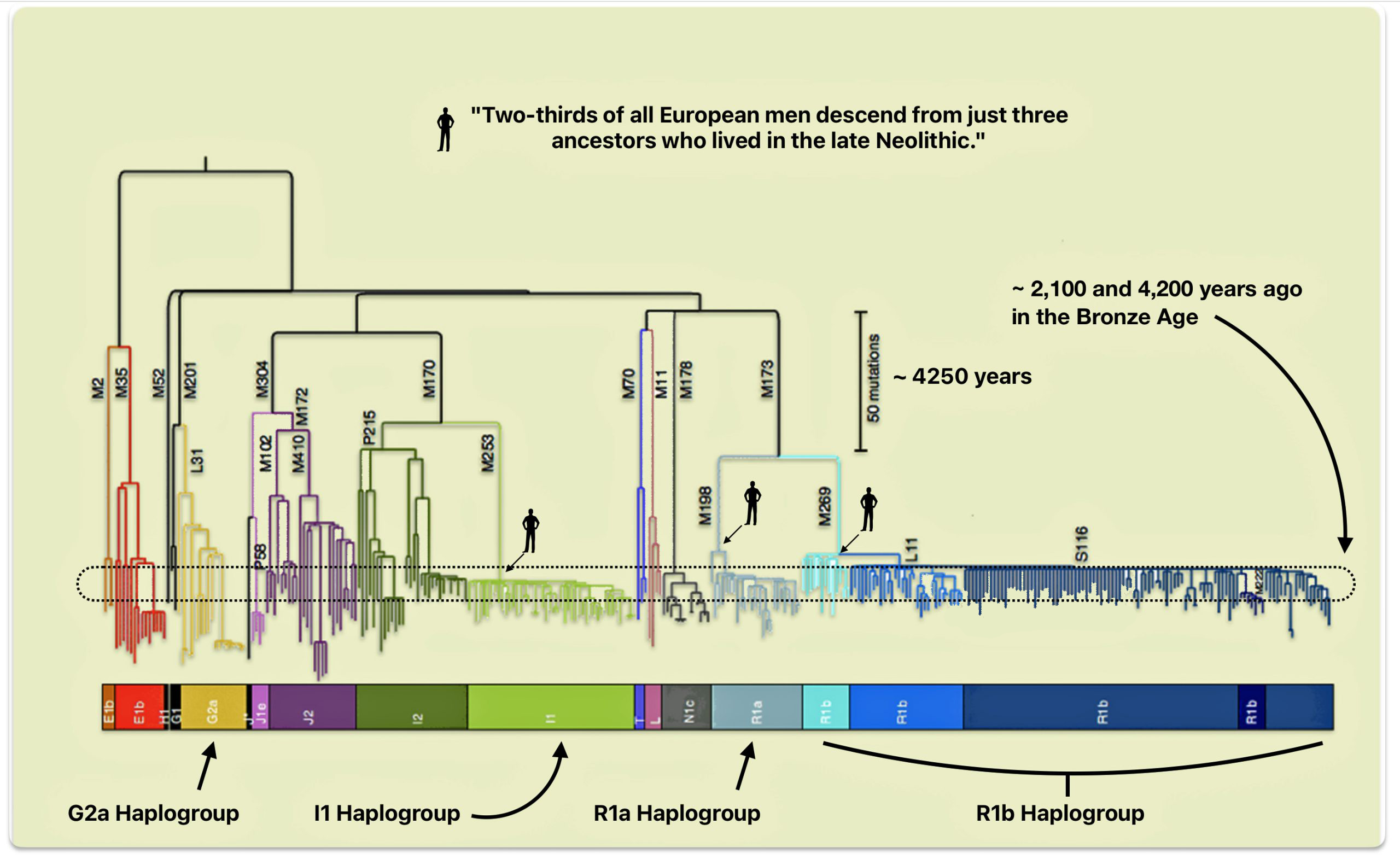
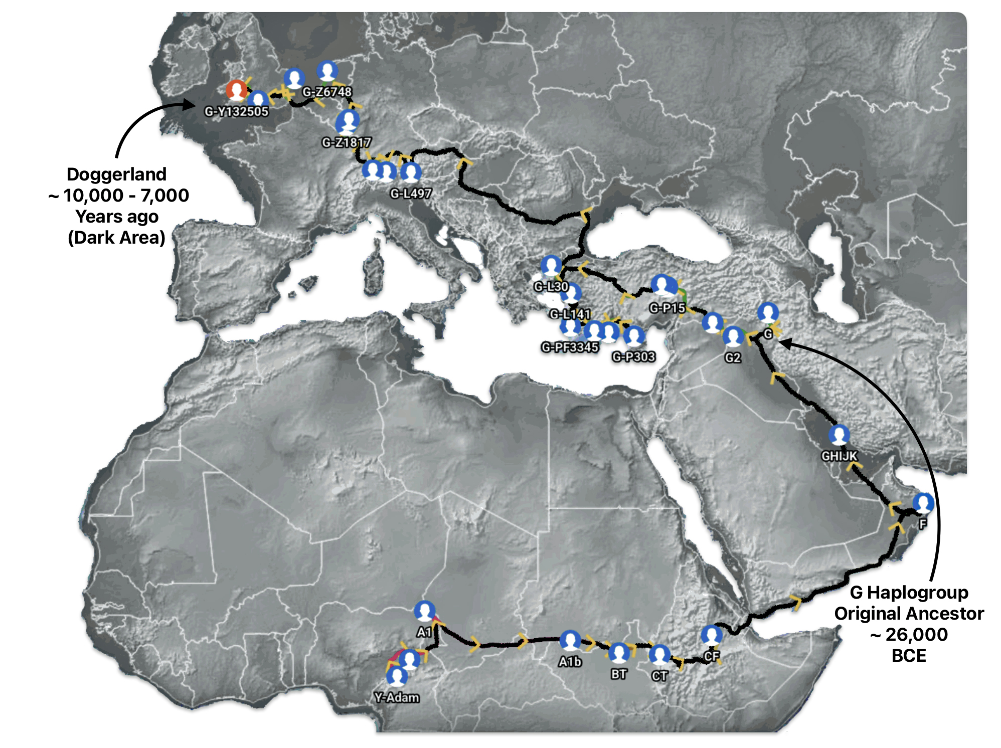
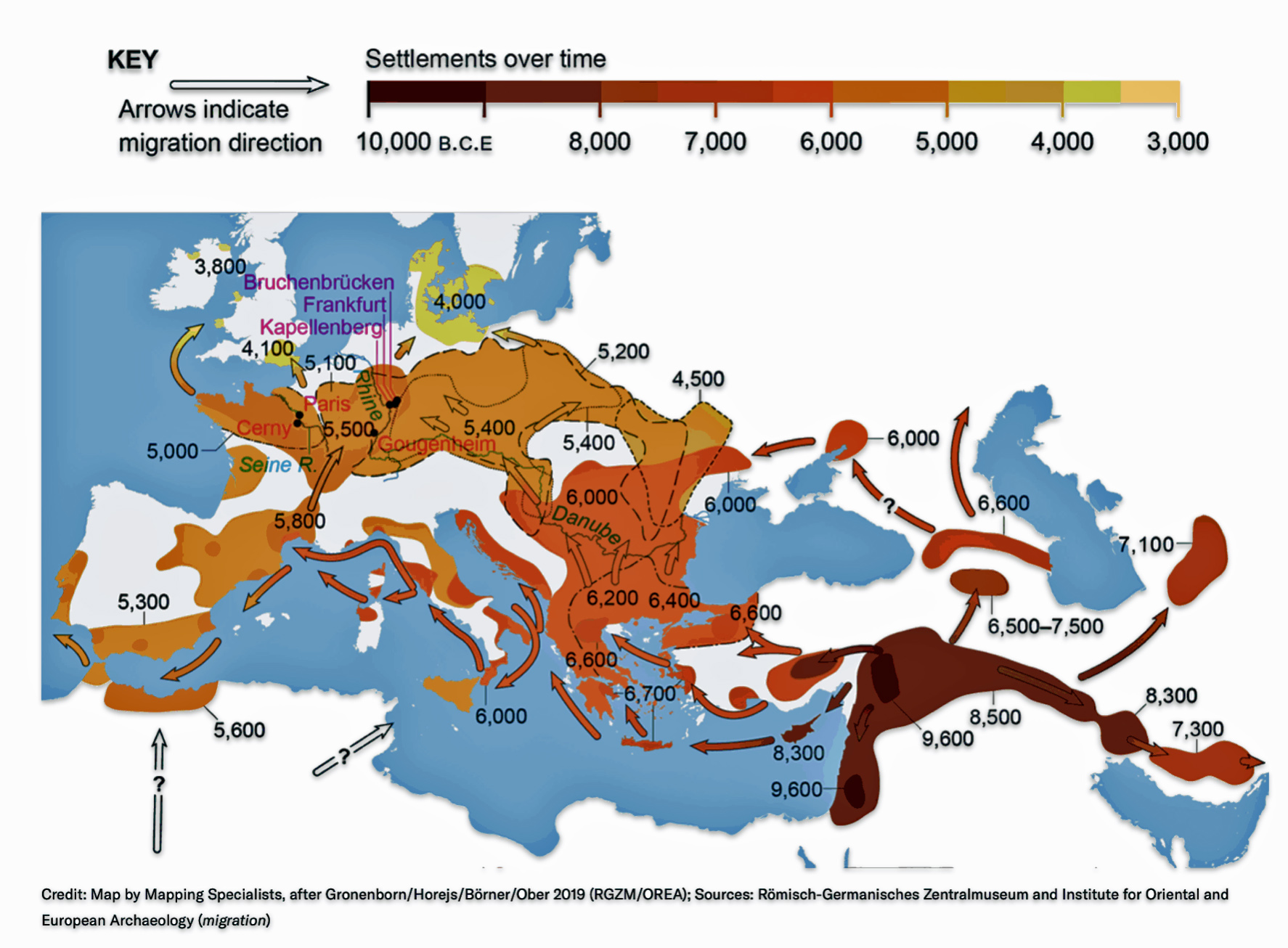
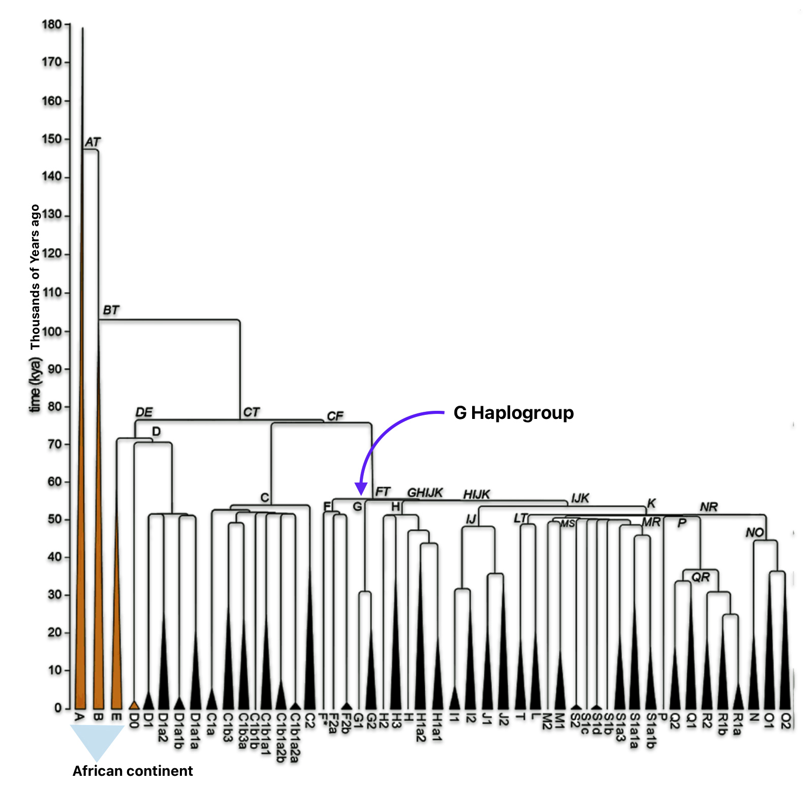
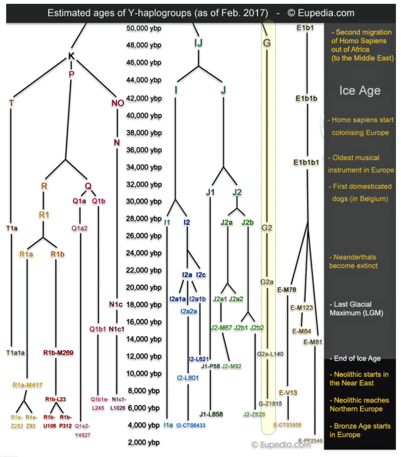
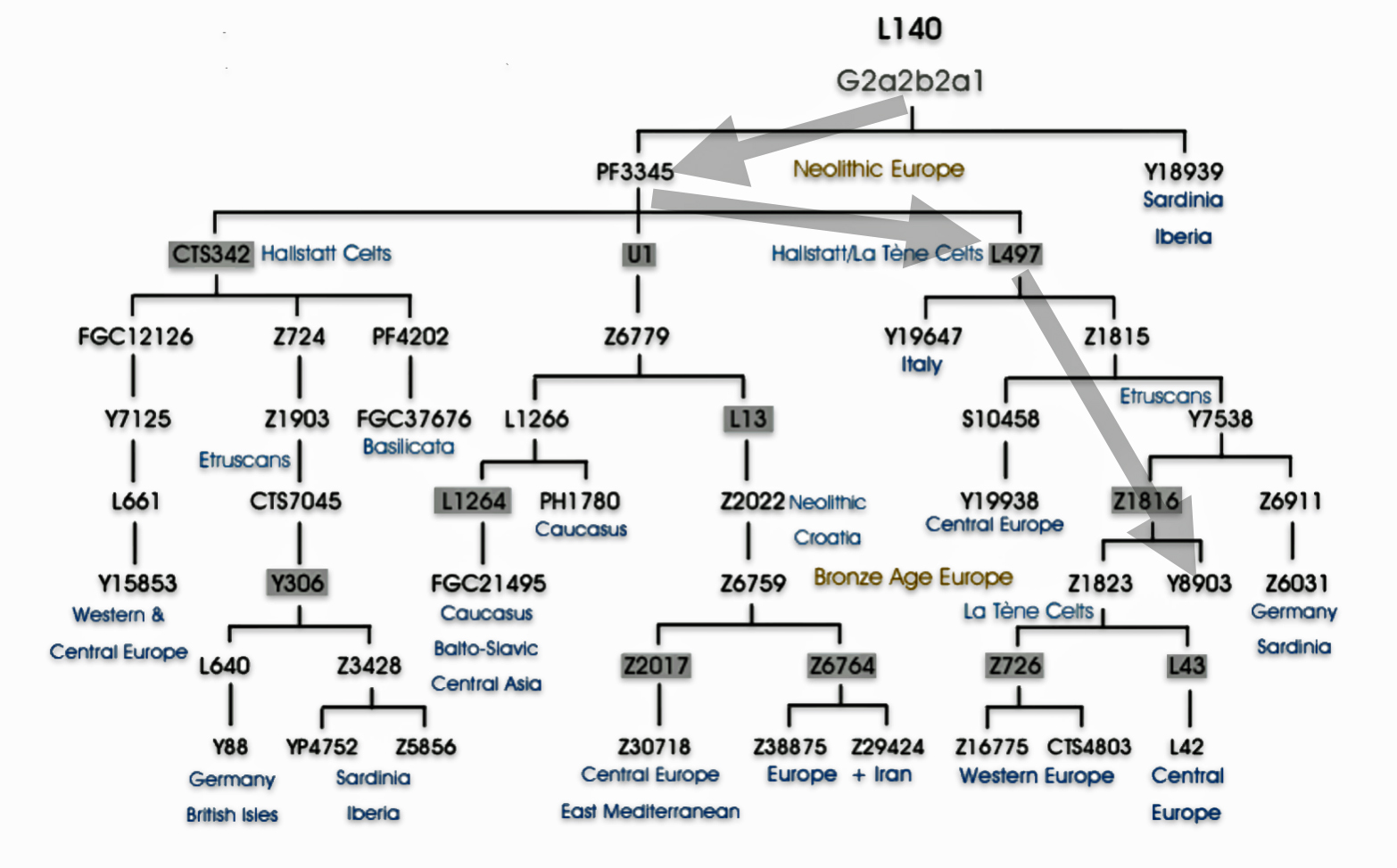
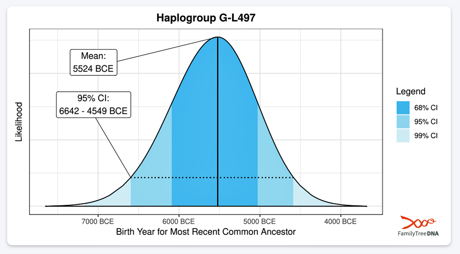
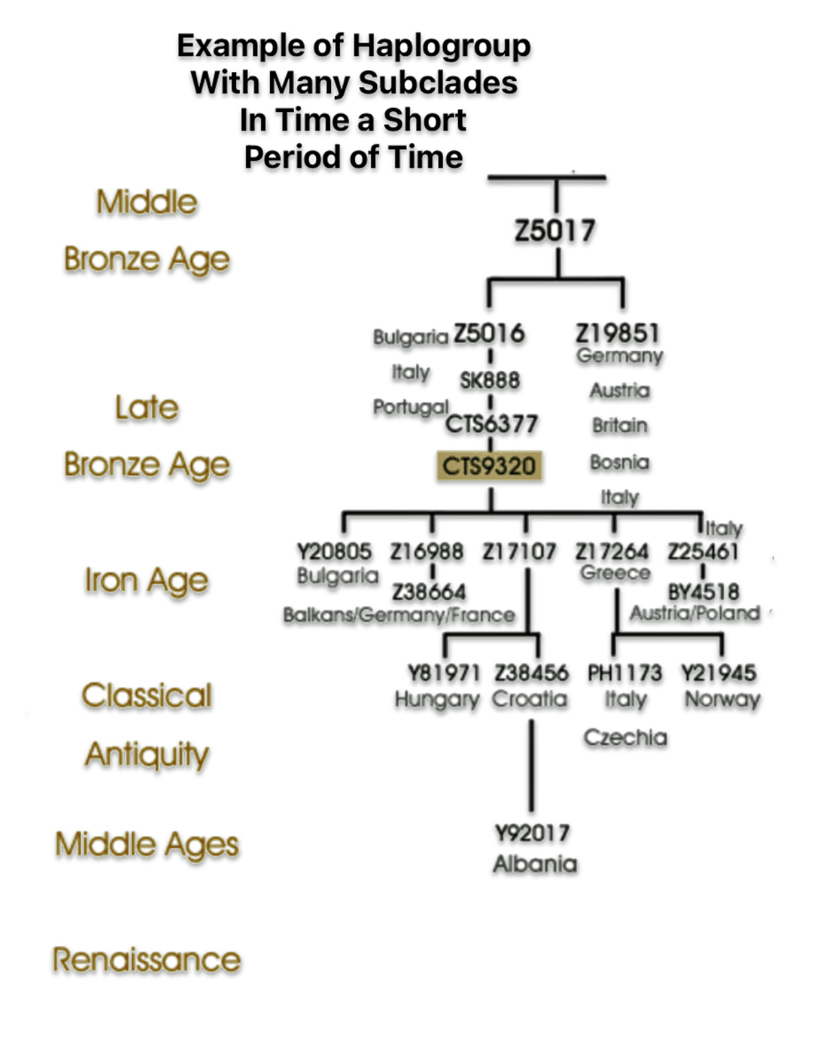
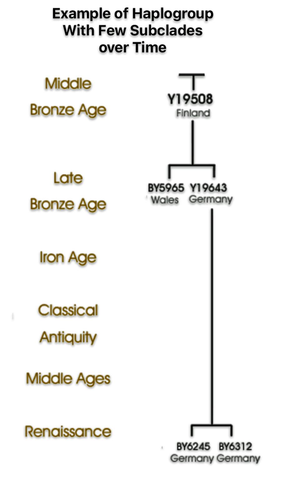
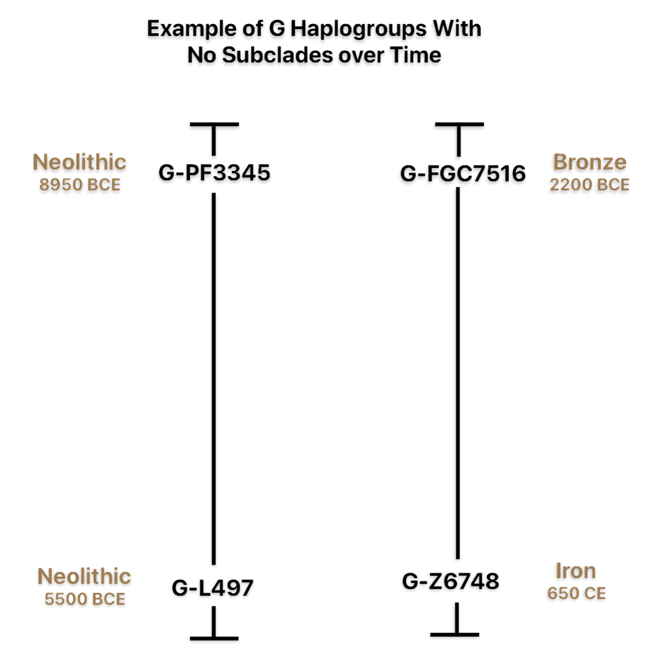
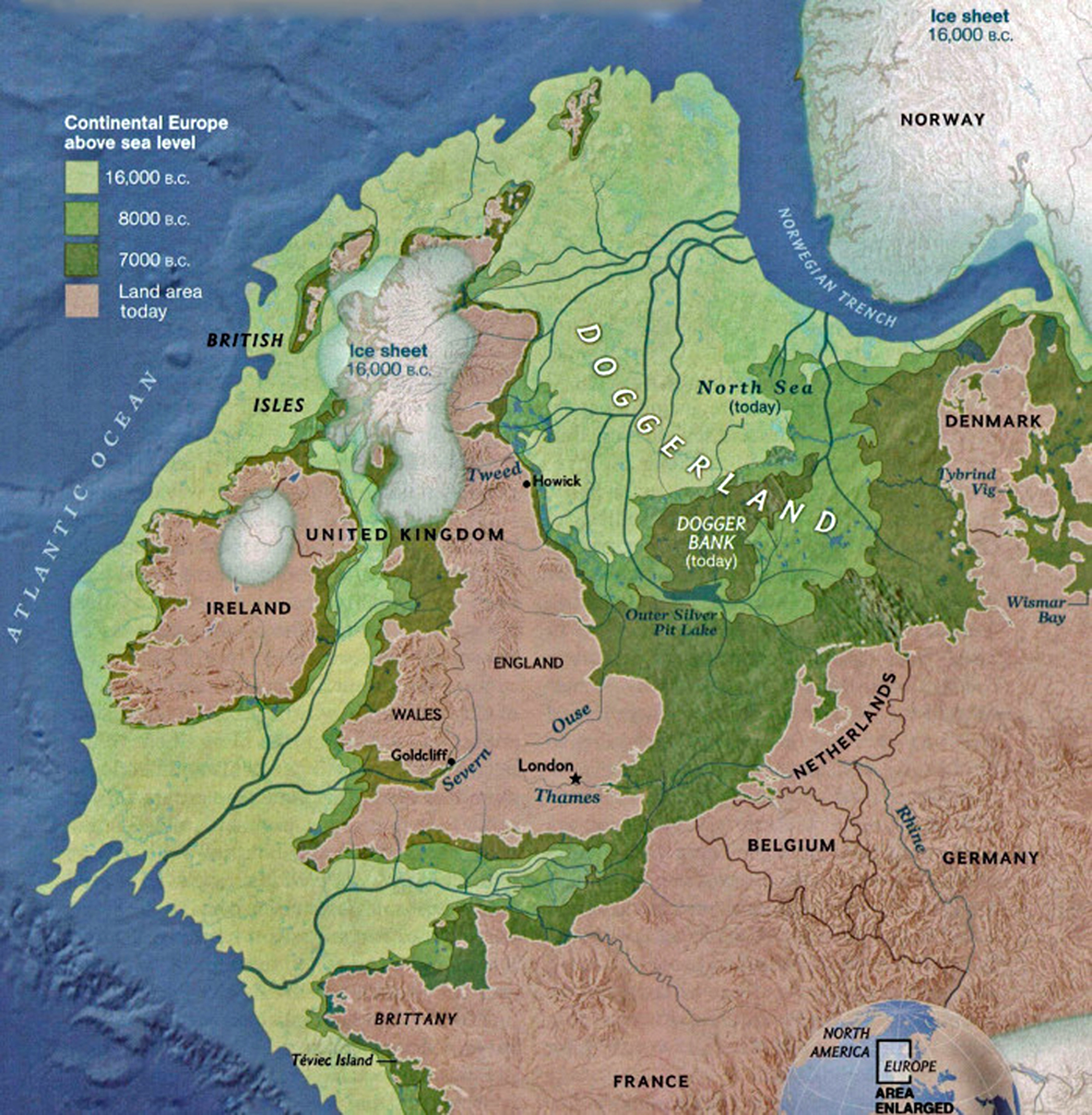
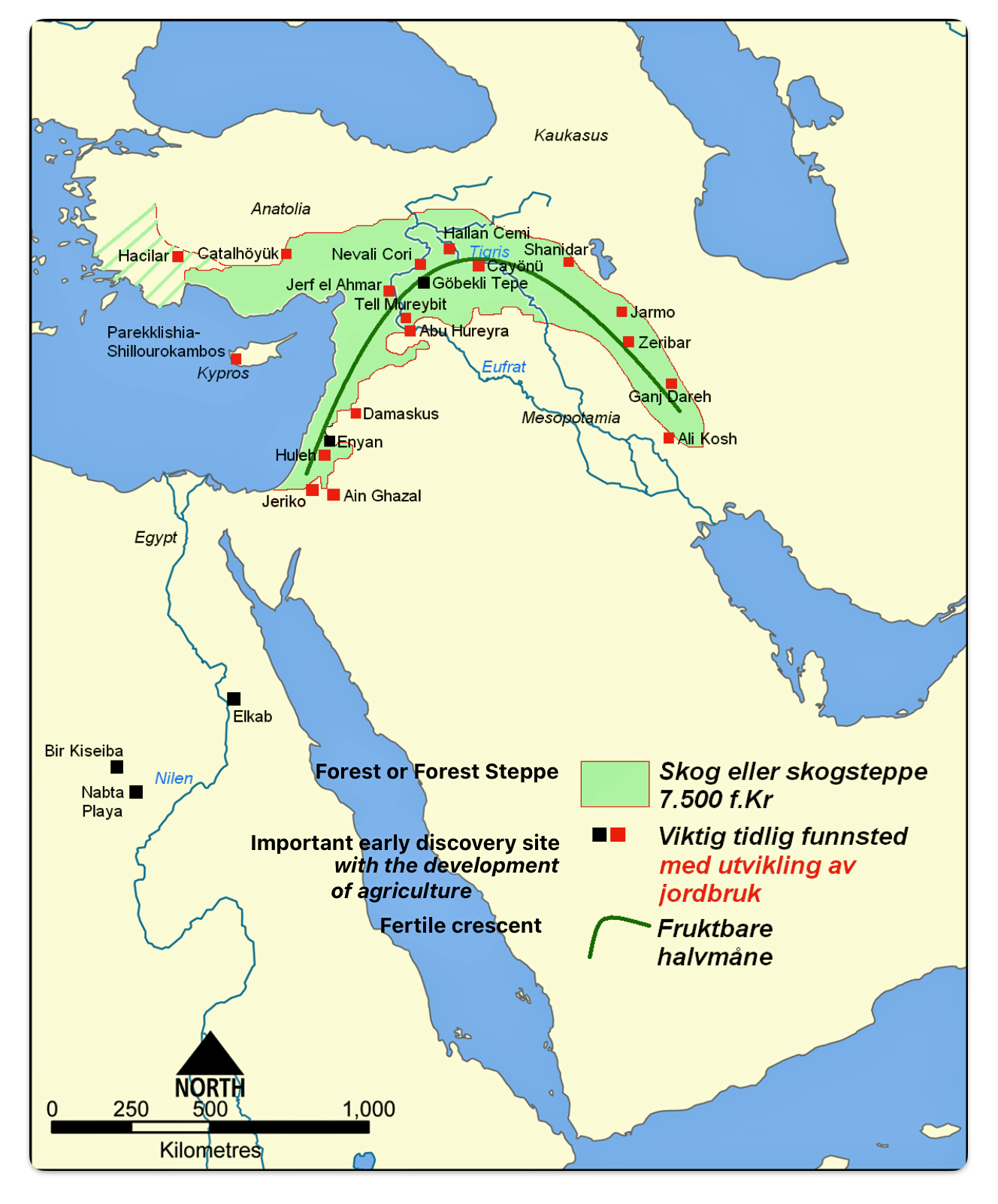
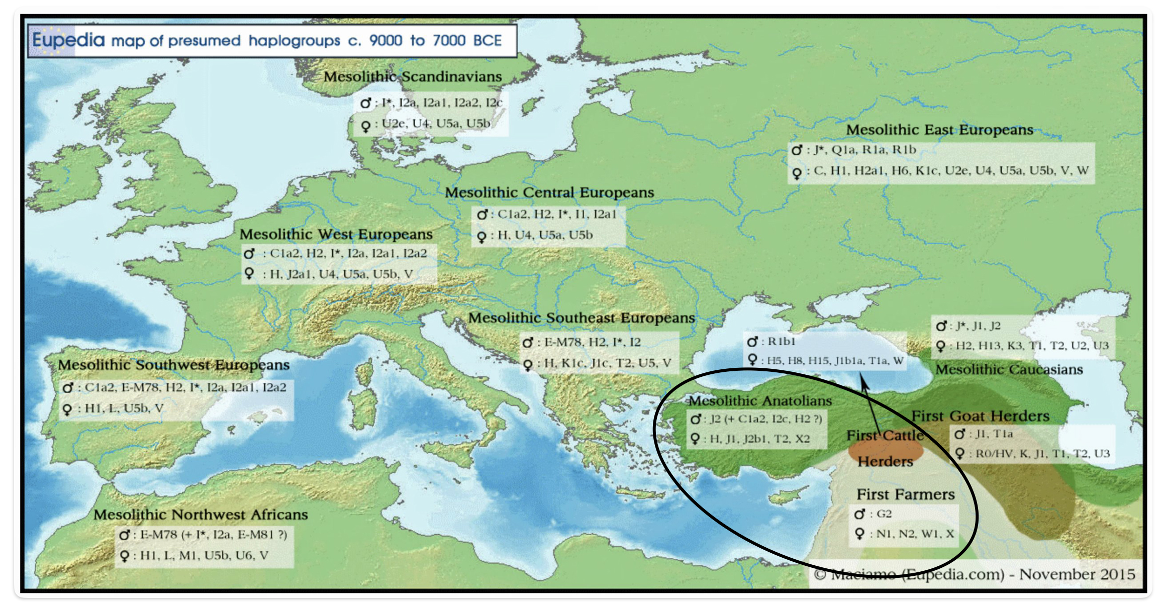
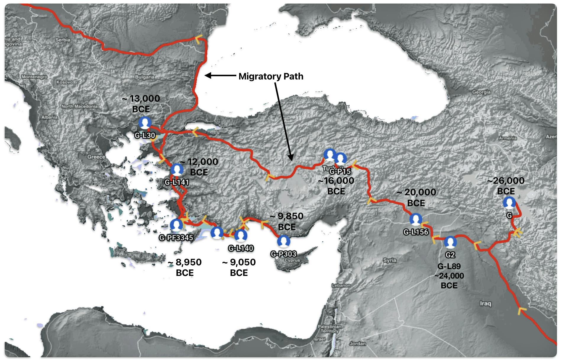
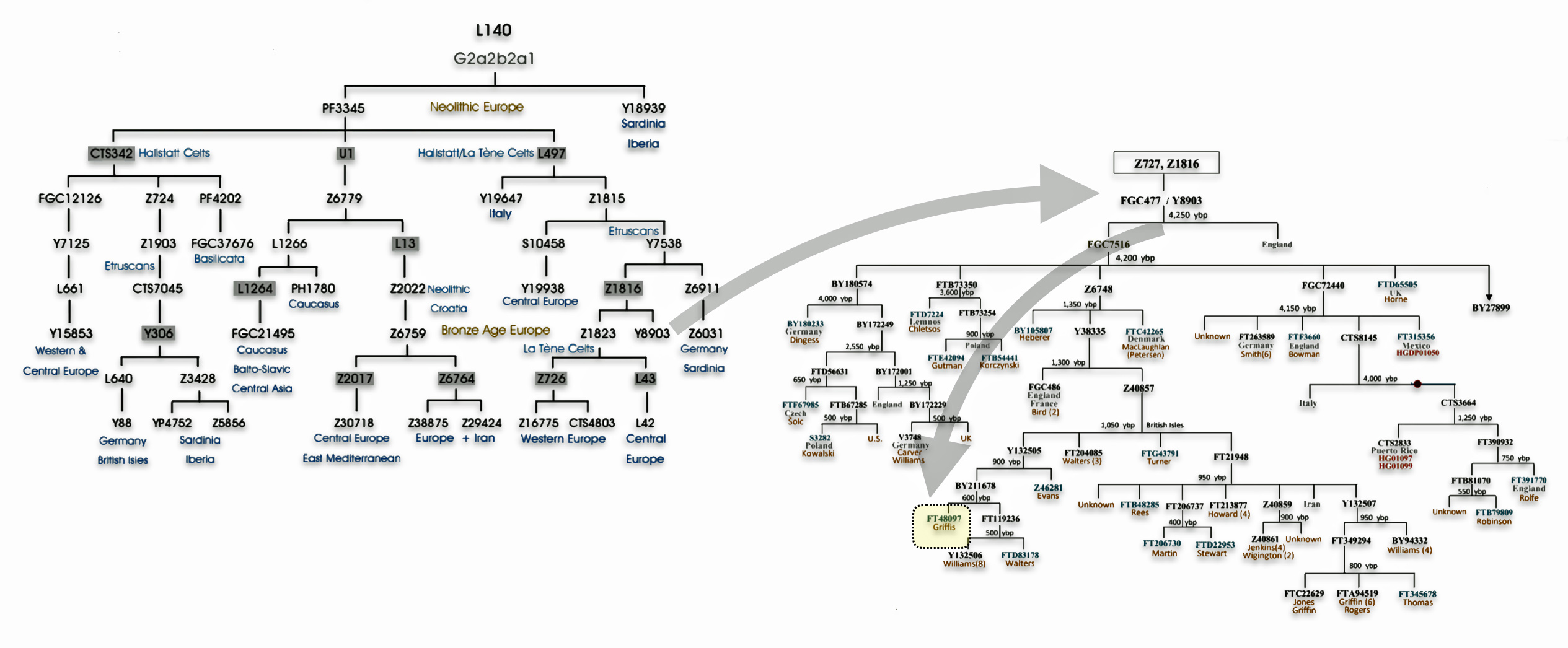