
It has been reported that “genealogy is the second most popular hobby in the U.S. after gardening … and the second most visited category of websites, after pornography. It’s a billion-dollar industry that has spawned profitable websites, television shows, scores of books and — with the advent of over-the-counter genetic test kits — a cottage industry in DNA ancestry testing.“ [1]
Since we are talking about the need for method and research standards, the veracity of the above quote has actually been called in to question by amateur genealogists. Time magazine, USA Today, Marist Opinion Polls, ABCNews, and other news sources who quoted this statement do not include general sources to back up their statement of fact about the popularity of genealogy. They also do not define what is a “hobby”, which would then allow one to determine the baseline for their statistics. The popularity claim appears to be an example of an unsourced statement that gained credibility through repeated citation rather than actual evidence. Consequently, the oft quoted statement about the popularity of amateur genealogical research is largely based on conjecture. [2]
“Observations about an American genealogy or family history boom have, however, been made many times before, such as in the 1920s and 1970s. Given its impact and longevity, it is safe to say that genealogy constitutes one of the most important sociocultural pursuits in modern U.S. history.” [3]
It is safe to say since the 1990’s there has been an appreciable increased interest in genealogy. The popularity of genealogy has been overstated, though it remains a significant interest, with seventy percent of Americans considering it important to know their family history. A recent poll finds that 7 in 10 Americans think it is important to know their family’s history. The poll also finds that older generations are more likely than younger generations to say that knowing their ancestry is important. [4]
More folks are interested in finding out about the past, their family ties and DNA connections. Much of the interest is attributed to access to digitalized genealogical records on the internet. The interest in genealogy is also the result of the availability of various DNA genetic tests to locate relatives and gain estimates of one’s purported ethnicity.
Consequences of Genealogy’s Popularity
The democratization of genealogical research has indeed created significant research quality concerns. It represents a double-edged sword – while making family research more accessible, it has also created significant challenges in maintaining research standards and accuracy. [5]
Amateur genealogists often perpetuate debunked theories and transcription errors through online sharing. The proliferation of undocumented genealogical research spreads like a virus as people incorporate unverified information into their family trees. An example of this is depicted in an online threaded discussion on John ap Gruffudd (Pengruffwnd) – Wales, an individual I will discuss below. One of the commentators of this ongoing discussion has labeled these family trees as “The Welsh Trees R Us”. [6]
The relationship between academic historians and amateur genealogists became strained, with some scholars dismissing genealogical research as lacking academic rigor. The “free and public” nature of online genealogy has led to concerns about the quality of historical material being co-opted by commercial sites. [7]
While digital technologies have made genealogy more accessible and affordable, this has created issues with data validation and verification. The genealogical industry’s promotion of easy access has contributed to a “genealogical craze” that sometimes prioritizes quantity over quality. [8]
“Web-grown genealogists are largely unschooled in research principles. Some learn quickly by devouring knowledge as well as names; but vast numbers remain untutored in the critical analysis of evidence and enthralled by some illustrious ancestry claimed for their “family name.” Unfortunately, they are also empowered with electronic tools that permit them to broadcast—instantly and word-wide, for other neophytes to replicate—an endless galaxy of mangled identities and supernatural trees rooted in the murky wonderland of cyberspace.” [9]
A major challenge for genealogists is to avoid falling into a trap of forcing facts, evidence of ‘common descendants’ into their desired view of the past and into their genealogical trees. There is a tendency among amateur genealogists to latch on to those few sources of available information about individuals in the distant past and attach them to their genealogical lineage without critical analysis.
These ‘common family’ ancestors become the ‘Adam or Eve’ of many family trees. This is especially the case with internet based family trees. This tendancy, howver, existed before the advent of commerical based family trees. Prior to the emergence of internet based family research, amateur genealogists would latch onto ‘prominent individuals’ that were mentioned in published manuscripts of families or surnames to build out their family histories.
The predominant reason why these individuals are referenced in so many disparate, unrelated family trees is mainly due to the simple archival fact that specific documents about these individuals have withstood the test of time and have not perished. Conversely, there is an absence of information on the other countless souls with similar names. Rather can declare that there is no evidence and that there is a brick wall in their family trees, researchers grab onto facts that provide no evidence of what they are attempting to prove.
The Griffis(ith)(es) Family Name from Huntington, New York
Reviewing and analyzing evidence found in genealogical work on the family surname through Griffin(th)(ths)(es)(ing)(s) family lineages in America had led me to question the validity and veracity of many of the genealogical stories, family trees, unpublished manuscripts, and published documents. [10]
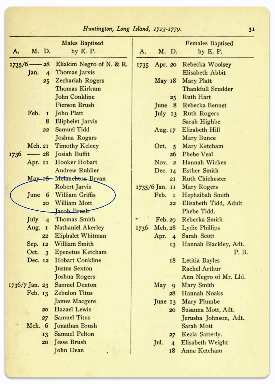
Derivative Source of the Baptism of William Griffis, My ‘Brick Wall’ for the Griffis Family
See related stories that touch on a critical analysis of genealogical studies on the Griff(is)(ith)(es) surname:
- Recent Discoveries from Oral History Compiled by a Local Mayfield Historian – Part I March 28, 2024
- Is the Huntington NY Griff(is)(es)(ith) Family Name Welsh? March 17, 2023
- Part Three: How Do You Spell Griffis? April 2, 2022
- The Griffis Surname and the Family from Huntington, New York: Part Two March 16, 2022
- Griff(is)(in)(ith)(iths)(es)(in)(ins)(ing) Surname and American Genealogies: Part One February 17, 2022
The Need for Verifying Evidence for Family Ancestors
The author of one self published manuscript on a Griffith family claimed: “To my knowledge this is the first book published with a complete pedigree of this Griffith lineage from year 100 through 1979.” [11]
Tracing one’s ancestors back to the year 100 CE is indeed a daunting and remarkable task that perhaps raises more questions concerning the veracity of sources. Many of the documented pedigrees of Welsh families in the medieval times that family genealogists rely upon were of gentry and nobility. Most of the ‘common folk’ were tenant farmers and while many took the names of the gentry that they worked for or lived nearby, it is highly likely the documented pedigrees are not their pedigrees.
It is a good example of why research standards should be followed when conducting genealogical research. The Genealogical Proof Standard (GPS) embodies the general research standards that conform to my personal research standards when conducting genealogical research.
The Genealogical Proof Standard (GPS) was developed by the Board for Certification of Genealogists (BCG) in the 1990s and was first formally published in 2000 in “The BCG Genealogical Standards Manual”. The standard was created in response to the booming internet era to help researchers navigate the challenges of online genealogical research and establish reliable proof standards. Before 2000, genealogists, such as myself, borrowed standards from other professions until BCG published their own list of genealogical standards. [12]
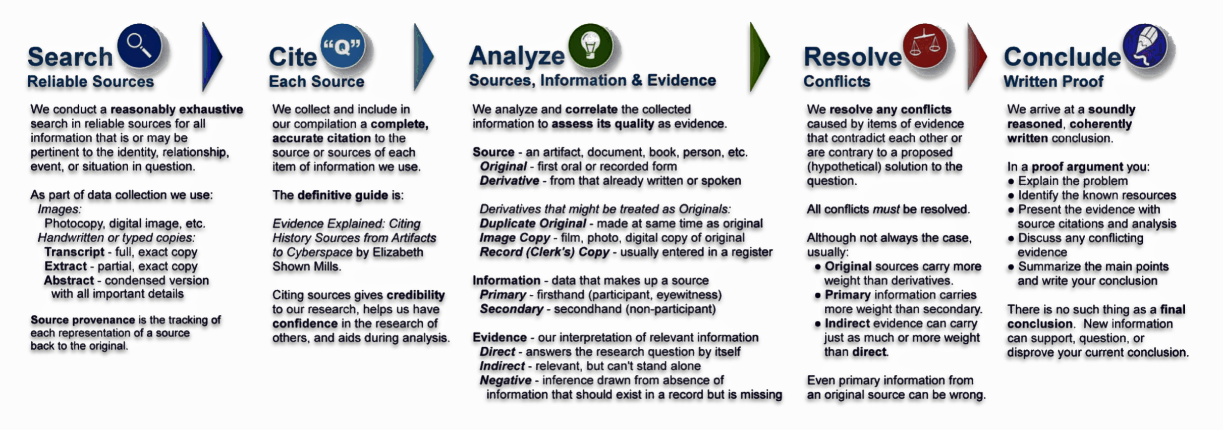
It serves as a methodology for both professional and amateur genealogists to validate their research findings. [13] As discussed in a prior story on genealogical facts and evidence, It consists of five elements:
- Reasonably exhaustive research;
- Complete and accurate source citations;
- Thorough analysis and correlation of evidence;
- Resolution of conflicting evidence; and
- Soundly reasoned and coherently written conclusion
Illustration One: The Genealogical Proof Standard
Common Myths and Unsubstantiated ‘Facts’
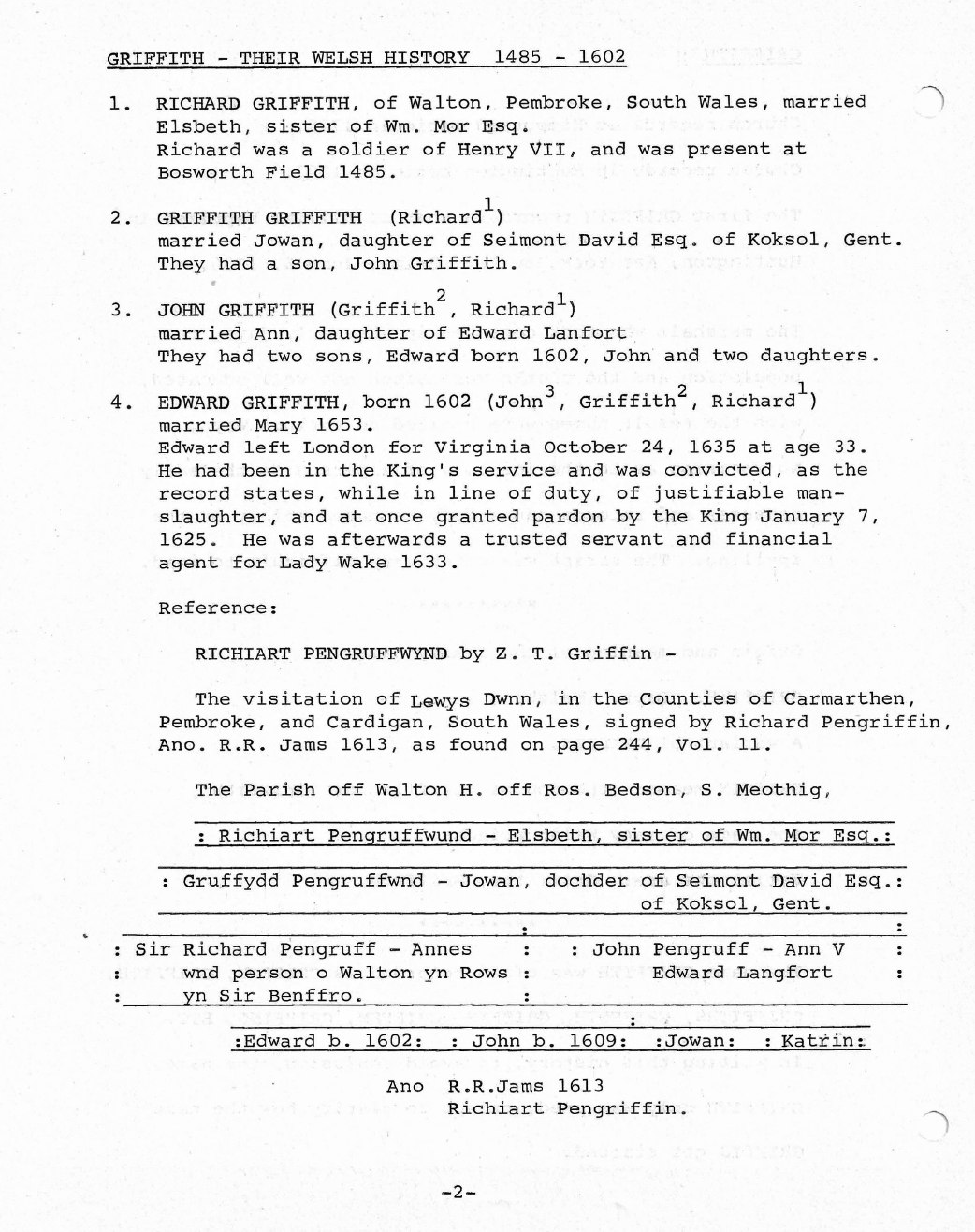
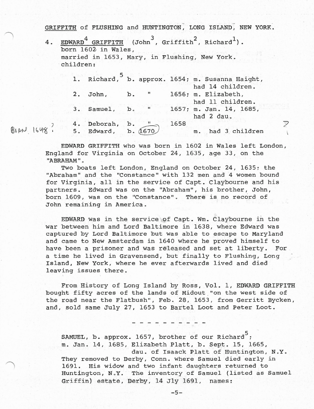
One of the common ‘myths’ or unsubstantiated series of facts that has repeatedly been used to build American Griff(is)(ith)(es) family trees is tying their family stories to the lives of Edward Griffin(en)(th) (born around 1602) and his brother John (born around 1608) from Walton, Pembrokeshire, South Wales. Depending on historical references, Edward and brother John’s last name is spelled Griffen, Griffith or Griffin. Both brothers purportedly traveled in 1635 from Wales on the ships Abraham and Constance respectively, landing on Kent Island off the coast of Virginia. They have been mentioned in various family manuscripts and published genealogies. If you start to research on any variant of the ‘Griff-‘ name in America, you will eventually be brought to these brothers. [14]
Many of the family histories also trace the purported family lineage backward from Edward Griffiin(en)(th) to Richard Pengruffwnd. This link is largely based on the research by Zeno Griffen. The common theme of this genealogical story is: Richard or Richiart’s descendancy purportedly is to a Gruffydd Pengruffwnd (Griffith Griffith) his son, who had a son John Griffith (who married Ann Langfort(d), who had Edward (b. 1602) and John (b. 1608). [15]
As Theresa Griffin, an amateur genealogist, has exhaustively and methodically documented in her research of the Griffin family, there were more than twenty Griffin family histories at the time of her critical analysis of Griffin family research that tie Pengruffwnd [Pengriffin] and his descendants with the Edward Griffith(in) who arrived in Virginia in 1635, and who ended his days as Edward Griffin(en)(th), in Flushing, New York. Almost all of these publications and family trees cite the written work of Zeno T. Griffen or can be traced back to his research. [16]
Through her methodical research Theresa Griffin cogently calls to question many of the assumptions, historical narratives, and family ties associated with Edward Griffin(en)(th), particularly the influence of the writings of Zeno Griffin. However, she perceptively acknowledges the limitations that professional and amateur genealogists faced before the advent of the internet and the digitalization of records, and the search accessibility of records that are common today.
“It is not my intention to condemn the work of Zeno T. Griffen, or any Griffin family historian. According to Zeno, he had relied upon his father’s unpublished, handwritten manuscript which was written circa 1830. The fact that Zeno was able to locate as much correct information as he did, without the use of the computer, Internet, easy travel, or on-demand access to documents from all over the world, is to be admired. I do not believe Zeno intended to deceive anyone with his suppositions, only that he had access to a small pool of documents and he drew his conclusions solely from that pool. … Although Zeno often gave specific dates for the events he reported, which was probably enough to convince early 20th century readers of his conclusions, with few exceptions he did not accurately cite his references. Because the current conventions for documenting sources are much more rigorous than they were in 1906, and access to ancient documents is on the rise, it is time to authenticate the facts presented in previous Griffin family histories.” [17]
Quality of Evidence in Family Trees and Manuscripts
There are a number of web based family trees, unpublished personal manuscripts and published sources that directly reference William Griffis(th)(in)(ths) of Huntington, New York. Five notable limitations for all of these web based trees and the family manuscripts are:
- None of the family trees provide complete lines of descendants for William’s twelve children that had families;
- All of the family trees lack sound, corroborating facts that support the linkages to William’s purported parents or grandparents and other ancestors;
- There is a general lack of citations for sources of evidence;
- Many of internet based family trees contain inconsistent or contradictory facts; and
- All of the family trees list family members with the same uniform surname with no substantiation of facts regarding discrepancies in spelling or that a given family member used a specific spelling of Griffis, Griffith, Griffies, or Griffes.
There are three genealogical manuscripts that explicitly mention William Griffi(th)(is) of Huntington, New York. Two of the manuscripts are unpublished. The third has been published by third party companies and may have been used to document facts in one of the other two manuscripts. [18]
Table One: The Three Manuscripts Related to William Griffis
| Manuscript | Description |
|---|---|
| Peets – Welsh Manuscript | Undocumented references to ancestors of William Griffis. Lists William and Abiah and 12 children, and descendants of second oldest son James. |
| M. K. Hall manuscript | Undocumented references to ancestors of William Griffis. Lists William and Abiah and 12 children, limited information on descendants of second son James. |
| Jones – Welch Manuscript | The Jones-Welch manuscript provides a wealth of information on the family tree of the fourth child of William Griffis: William Griffis who was born in 1763. |
Similar to the other manuscripts and published works about the Griffin family surname previously mentioned, they exhibit similar patterns of linking individuals without genealogical proof or citations prior to the early 1700’s.
One of the three manuscripts, which I refer to as the “Peets-Welch manuscript“, based on the author’s names, gives credit to the work of Martha K Hall. Hall was the historian for the Huntington Historical Society when Mildred Griffith Peets was writing her manuscript. Much of her research on the early descendants relies on Hall’s research and manuscript. The Peets-Welch manuscript provides information found in earlier “Griff-” family manuscripts about the purported origins of the family as well as more detailed information on James Griffis, the second oldest child of William, and his descendants.
The Peets-Welch manuscript relies on the purported ‘facts’ that were referenced in prior published Griffin family research, attempting to tie the family lineage back to Edward Griffiin(en)(th) to Richard Pengruffwnd (see below). In addition, the principal author, Mildred Griffith Peets, attempts to link an Edward Griffith(in) with a Richard Griffith who in turn purportedly had a son named Samuel Griffith(in). Her documentation is sketchy, disjointed, and citations for linking each of the individuals is absent. The manuscript is written in a fashion that resembles working notes for research leads.
Pages from the Peets-Welch Manuscript Illustrating ‘Leaps of Faith’ Regarding Family Ancestors
“Griffith – Their Welsh History”
“Griffith of Flushing and Huntington”
Another manuscript, the ‘Jones-Welch manuscript‘, provides a wealth of information on the family tree of the fourth child of William Griffis: also named William Griffis who was born in 1763 and died in 1847. What is interesting about William Griffis is after serving in the American Continental Army in the American Revolution, he emigrated to Canada as a loyalist.
While these Griffis(ith) manuscripts may have certain limitations or gaps in facts and documentation, they are useful documents that provide insight into our Griffis family from Huntington, New York. They document specific branches of the family tree not only in New York state but in other parts of the country as well as Canada. They, however, have no information on my specific branch of the Griffis(th)(es) family ( the descendants of Daniel Griffis) or other branches of the family.
I continue to rely upon the above mentioned manuscripts for further leads in research. Their intentions for genealogical research were genuine but their ability to seek answers to their research questions were limited and perhaps were justifiably focused on a particular branch of the Griff(is)(ith)(es) family.
Access to genealogical sources were much more limited prior to the advent of the internet era and digital records. However, the conventions for documenting and citing sources, which are much more rigorous than simply citing an assertion or hearsay quote from a relative, call for the need to validate, in some fashion, the facts presented in previous family histories.
In Support of Research Standards
The lack of critical analysis, citations for facts and evidence in manuscripts, books and online research about the Griff(is)(ith)(es) family underscores the need for an increased emphasis upon documentation, adherence to research standards, an analysis of facts and evidence, and record interpretation. A critical eye, a set of research principles to guide you and various methodologies to objectively analyze the facts are needed to sift through all that is posted on the internet and found in paper documents.
Guided by research standards resembling the above mentioned Genealogical Proof Standards and using traditional genealogical and historical methods, combined with Y-DNA genetic testing and methods:
- there is documented evidence of the existence of three variants of the Griff(is)(ith)(es) surname for the descendants of William Griffis in America;
- there is a possibility that William’s ancestors used Griffis, Griffith or Griffiths as a surname in Wales
- there is evidence of genetic patrilineal descendants in Wales that used other surnames; and
- there is strong evidence that the Griff(is)(ith)(es) patrilineal lineage came from the southern area of Wales and had been in Wales for a substantial period of time.
These new family research breakthroughs are partly the result of relying on the aforementioned work done by others and that facts about the family are discovered by building on previous discoveries. The results are also attributed to the ability to discover new evidence in digital form, published research on the Welsh patrilineal naming system and utilizing new discoveries and methodologies produced by contemporary researchers in traditional and genetic genealogy.
The Use of Surnames Based on Historical Documentation
If one understands the history behind the emergence of family names in Wales and the research benefits of Y-DNA tracing of the patrilineal line back through time, one should be receptive to the idea that surnames are not fixed and they are fluid through time. In fact, it is not uncommon to have different surnames associated with the same Welsh Y-DNA patrilineal family lines.
The use of surnames did not become widespread in Wales until the late eighteenth century. In the greater part of Wales, the ancient patronymic naming system continued: having children identified in relation to their father. This meant that surnames in the 1600’s and 1700’s, and even as late as the 1800’s, did not take on the weight of significance that they have for present generations. [19]
Map One: Patronymic Decay and the Rise of Surnames in Wales
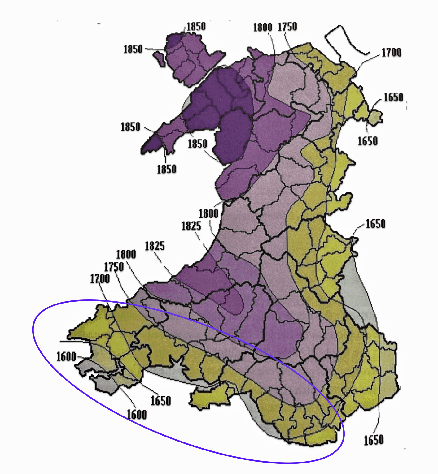
The map above (Map One), reveals the wide variation when surnames were adopted in various parts of Wales. Surnames became the norm by 1750 across the coastal plain of south Wales and along the eastern border with England. The Griff(is)(ith)(es) family line was probably from the blue circled area on the southern coast of Wales. The evidence that supports this supposition is discussed below.
It was not until the mid-nineteenth century that the Patronymic system was fully replaced in Wales. When the Welsh immigrated to America in the sixteenth and seventeenth centuries, the patronymic pattern on both sides of the Atlantic was in stages of decay. It is not uncommon to find variations of surname spellings within and between family generations. The use of surnames was, compared to the curing of concrete, “wet cement” in the 1600’s and 1700’s.
It was in this historical context that it was not a total surprise to document the use of three different spellings of the family surname in the mid to late 1700s. A review of the historical documentation and evidence associated with the different surname spellings can be found in a prior story. [20]
A variety of Federal, state and local records were used to determine the spelling patterns among the twelve children of William Griffis and their respective families. Baptismal records, marriage records, family manuscripts, burial records, cemetery records, church records, tax records, Federal and state census records, and revolutionary war records were used to document naming patterns.
Government records often can contain errors associated with names, dates and other information, so multiple pieces of corroborating evidence were gathered to assess naming patterns for each sibling of William Griffis and their respective family members. A strong genealogical proof relied on finding consistent information across multiple independent sources, not just relying on a single document.
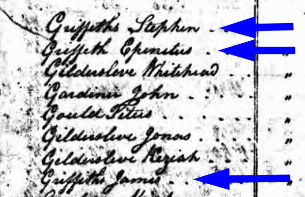
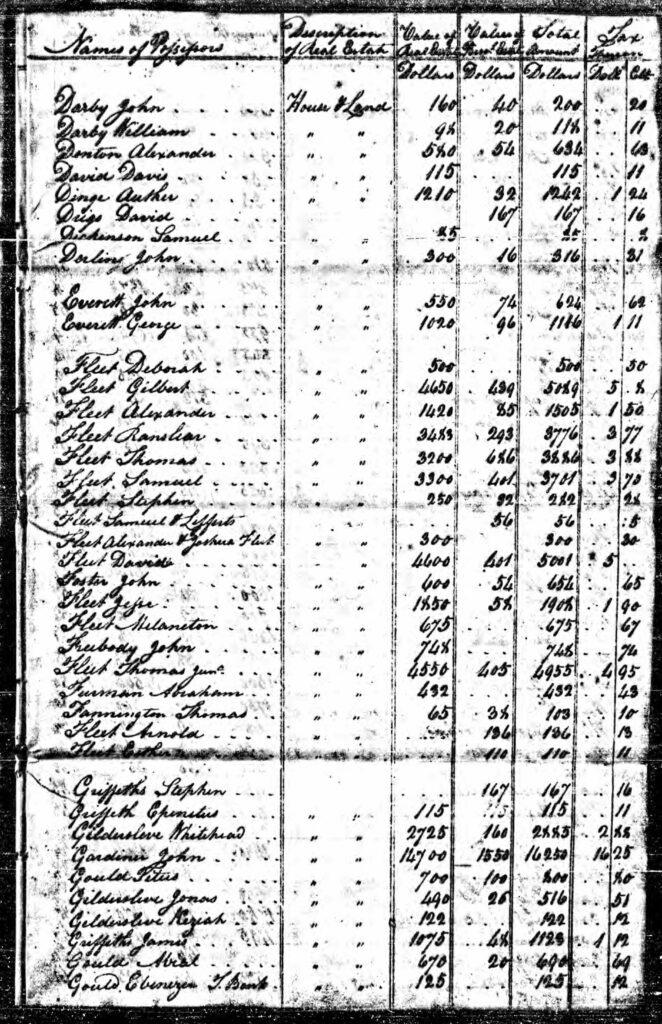
An example of the variability in transcribing individual information can be found in the Huntington, New York Tax Rolls. The surname is spelled as Griffeth, Griffeths, and Griffiths. In 1799, the tax assessors located three of the brothers. I imagine the enumerator of the tax information probably knew the three ‘Griffis’ brothers since it was a small community. Nonetheless their names were spelled three different ways: Stephen Griffeths, Epenetus Griffeth, and James Griffiths! [21]
Huntington, New York Tax Rolls, 1799
Various ‘correlation tools or methods’ were used to analyze and compare different pieces of information from various sources to identify patterns and confirm relationships between individuals and family members. The approach was essentially piecing together a family tree by looking for consistent details like names, dates, locations, and other identifying factors across multiple records, using tables, timelines, maps, and lists to visualize these connections. [22]
Illustration Two: William and his Twelve Children
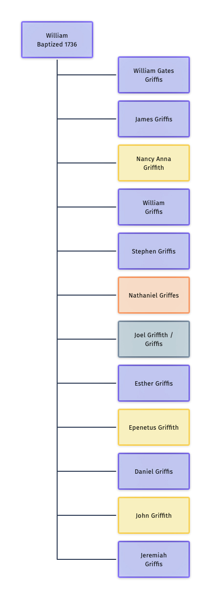
The chart to the left (illustration two) reflects the variations in spelling in the family surname among William’s 12 children.
Based on my assessment of genealogical evidence, seven of the children used the ‘Griffis’ surname, three used the ‘Griffith’ surname and one used the ‘Griffes’ surname.
The third generation of the family reflects a continuation of various spellings of the surname. The descendants of William’s second child, James Griffis, reverted back to the ‘Griffith’ surname. The descendants of the third son, William Griffis, used both Griffis and Griffith. Three of his four sons used ‘Griffis’ while a fourth son used ‘Griffith’.
The fifth son, Stephen Griffis, appeared to have used or was recorded as a Griffith and Griffis but it is not entirely certain what he actually used as a last name.
Nathaniel Griffes, the sixth son, was the only child that spelled his name as an adult with an ‘es’ on the end, Griffes. His descendants continued the tradition.
While it is not entirely certain, Joel Griffith probably spelled his name with a ‘th’ on the end.
Little is known of the second daughter of William, Esther Griffis, but she probably spelled her last name as Griffis.
Epenetus and John used Griffith and Daniel and Jeremiah used Griffis.
Using Traditional Genealogical Methods and Evidence: The Origin of the Patrilineal Family Line
Family oral history and family genealogy manuscripts suggest that the Griff(is(ith)(es) surname is of Welsh origin. There is a lack of solid traditional evidence that William’s ancestors were from Wales.
It appears based on oral history that either father or grandfather of William Griffis were the original family emigrants to the colonies. Contrary to a wide range of Griffin(th)(ths)(is)(es)(in)(ins)(ing) American family genealogies, William’s ancestors were probably not descendants of a Edward Griffin or a Richard Griffin. There are references to a Samuel Griffin (Grffing)(Greffith) (Griffith) who lived and owned land in Huntington Long Island in the late 1600’s but there is no definitive proof that he is William’s grandfather or father or was related to the family.
Oral history can be a powerful tool for historical research, if it is combined with other sources and methods. It is a form of evidence rather than an absolute truth. It can be used to complement and enrich other sources, such as documents or artifacts, by providing personal and contextual details. It can also challenge other sources by exposing gaps or contradictions, or by offering different interpretations or explanations. Oral history can create and contribute new sources by documenting and preserving the voices, stories, and experiences of people who may not be remembered otherwise.
There are also limitations that should be taken into consideration when evaluating the facts obtained through oral or written interviews:
- Memory and Recall Issues: Oral history relies on the memory of individuals, which can be influenced by time, age, trauma, bias, and other factors.
- Subjectivity: The formation is subjective and influenced by personal biases, which may lead to distortions or inaccuracies.
- Verification Challenges: There can be a lack of corroborating evidence, making it difficult to verify or cross-check information.
- Single Perspective: Oral histories often represent a single person’s viewpoint, which can lead to an incomplete or biased historical record.
- False Memories: Individuals may recall memories that actually different from what actually occurred, especially for events that occurred many years ago.
- Interview Dynamics: The relationship between the interviewer and interviewee can create dynamics that affect the narrative, the nature of questions asked and how answers are provided based on the context of the interview.
Family folklore indicates that Albert Buffet Griffith told his daughter-in-law, Lillian, that “his great, great grandfather’s name was Samuel“. [23] Albert was a descendant of William’s fourth child, William Griffith. If Albert Griffith’s recollections are true, then William’s father was perhaps Samuel Griffith(is).
I obtained copies of handwritten notes on the descendants of Daniel Griffis, William’s tenth child and my direct descendant. This branch of the Griffis family lived in Niskayuna and then Mayfield, New York in the mid 1800s through the 1930s. [24]
The three pages of handwritten notes were kept by a former Town of Mayfield, New York Historian, the Reverend Edward Ruliffson. Ruliffson’s notes were based on information he received in 1935. He interviewed William J. Griffis. William’s grandfather was Daniel Griffis and his great grandfather was William Griffis from Huntington. [25]
In his notes, Rulifson indicated “The name is Welsh, the same as Griffin. A Daniel Griffis came from Wales. About 1830 a Daniel Griffis, some generation or generations removed from the first Daniel came to Mayfield from Niskayuna where he married a Miss Gates and where he lived some years following his marriage.” [26]
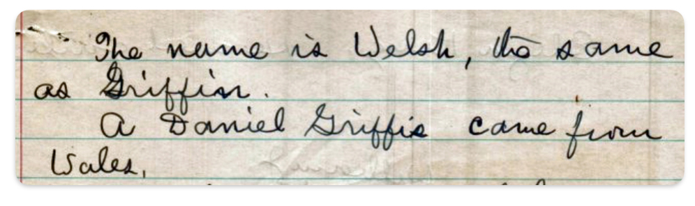
What is telling from the oral history transcribed by the local historian Rulifson is that purportedly a Daniel Griffis came from Wales and some generation or generations removed ,William’s son Daniel Griffis moved from Niskayuna to Mayfield, New York. This piece of oral history implies there is a generation or two prior to William Griffis that immigrated from Wales. It also implies there are two Daniel’s in he family tree.
If Albert Griffith’s recollections are true, then William’s father was perhaps Samuel Griffith. This does not refute Ruliffson’s statement that a Daniel Griffis came from Wales. Perhaps the father of Samuel, who purportedly was William’s father, was Daniel. This would imply that William Griffis(th)’s grandfather was the first generation to arrive in the colonies.
However, we have no corroborating proof to substantiate whether a Daniel Griffis(ith) came from Wales. We also do not have corroborating proof that William’s father was Samuel Griff(is)(ith).
Based on historical documents associated with colonial migratory patterns, William’s father or grandfather possibly came from Bristol, which is close to the southern border of Wales, to Boston or another northern port. They initially settled in Massachusetts or Connecticut as early as 1630-1640. The family then emigrated to Huntington as part of a series of emigrant waves to populate newly established English towns on Long Island.
The Use of Griffis(ith)(iths) Surname in Wales
The Griffis(ith)(iths) surname was used by families in various parts of the British Isles. The ancestors of William Griffis could conceivably have been from anywhere in Great Britain given the prevalence of the Griffi(th)(ths)(es)(s) surnames. Based on an analysis of census data in Wales in 1850, the top ten most common names represented approximately 80 percent of the Welsh population. While these names were common, it does not imply they were related. The result of using similar names as surnames resulted in the lack of diversity in surnames in Wales. [27]
A review of data from the 1881 census of Great Britain and Griffith’s Valuation in Ireland 1853-1865, indicate that the surname of Griffith and Griffiths is found in a large number of countries throughout Great Britain and Ireland. There is a good chance that the ancestors of William Griffis were from Wales and from southern Wales. Of course, this statement is based on the assumption that the 1853-65 and 1881 data sets may illustrate enduring trends in the distribution of surnames from the time William’s ancestors left Great Britain.
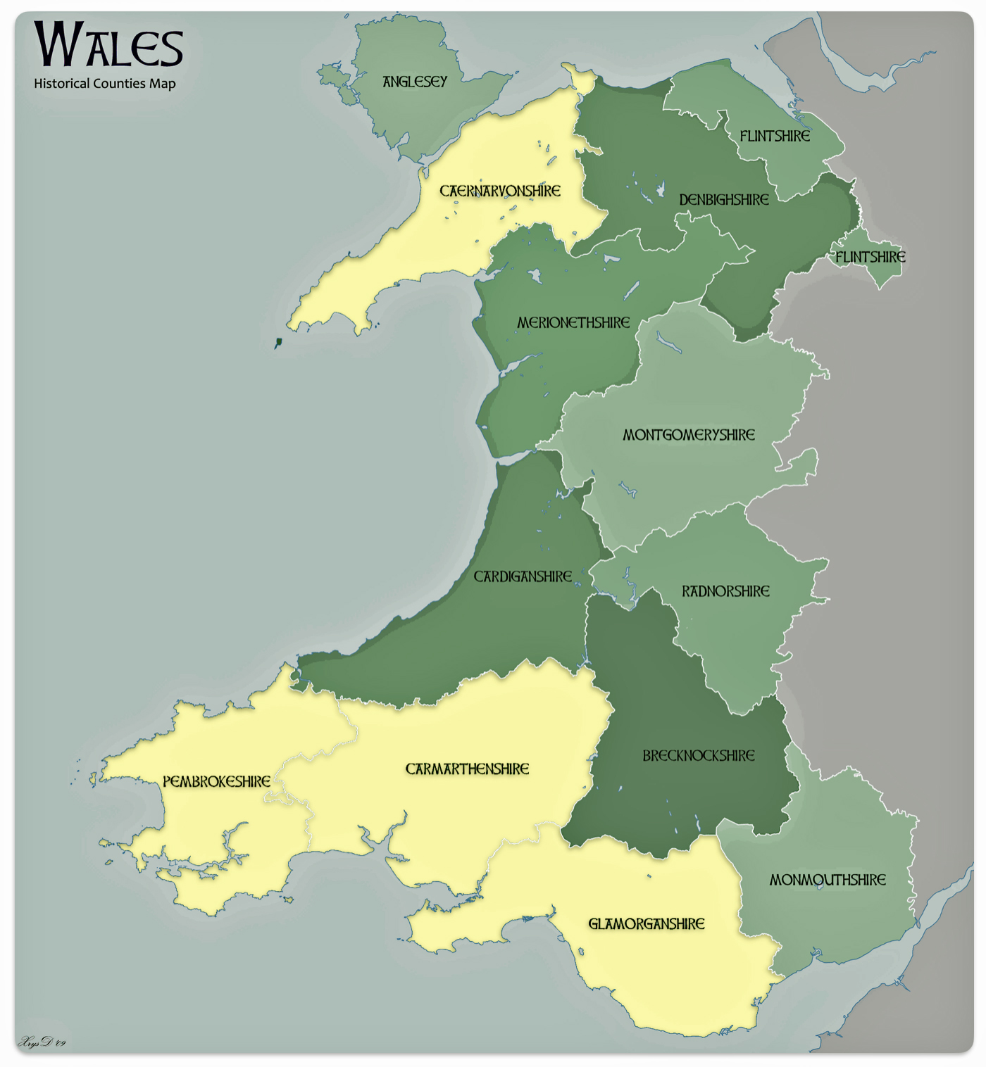
Four counties in Wales represent more than a majority of households with the name of Griffiths or Griffith. Perhaps William’s ancestors were from Glamorgan, Penbroke, Caernafon or Carmarthen counties. These four of the twelve counties represent 63 percent of Welsh households that have the name Griffith or Griffith. Glamorgan has the largest proportionate presence of the Griffith(s) surnames (27%). Penbroke, Caernafon and Carmarthen are the second, third and fourth largest in representation of Griffith(s) households (15.7%, 10.4% and 10.0% respectively). While these four counties contain the largest concentration of Griffith and Griffiths households, the Griffith(s) surnames are represented in all of the Welsh counties. These two surnames are in the top ten of most popular surnames in seven of the twelve counties. [28]
Map two provides a graphic representation of where the top four counties are located. Three of the four reside on the southern coastal border of Wales. Monmouth county, which is also on the southern border, also had a sizable proportion of households that had the Griffiths name.
Map Two: Welsh Counties with Concentrations of Griffith and Griffiths Surnames
Not only should variants of the spelling of a surname be considered when reviewing various census repositories of information, different surnames should also be considered in specific geographical areas. It is not inconceivable that individuals who were related at specific historical times may have decided to use different surnames when these of surnames became popular.
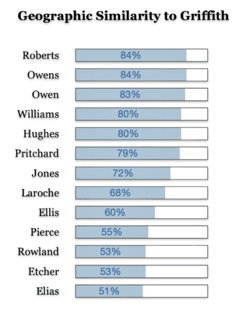
There are a number of Welsh surnames that are geographically similar to where Griffith(s) surnames were found in 1881. The common Welsh surname of Roberts, Owens, Williams, Hughes, Pritchard and Jones are found 80 percent of the time in counties where the Griffith(s) households resides (see below). This is not surprising given the that these surnames were found in most of the Welsh counties. What should be kept in mind is many of these families with these different surnames could be genetically related.
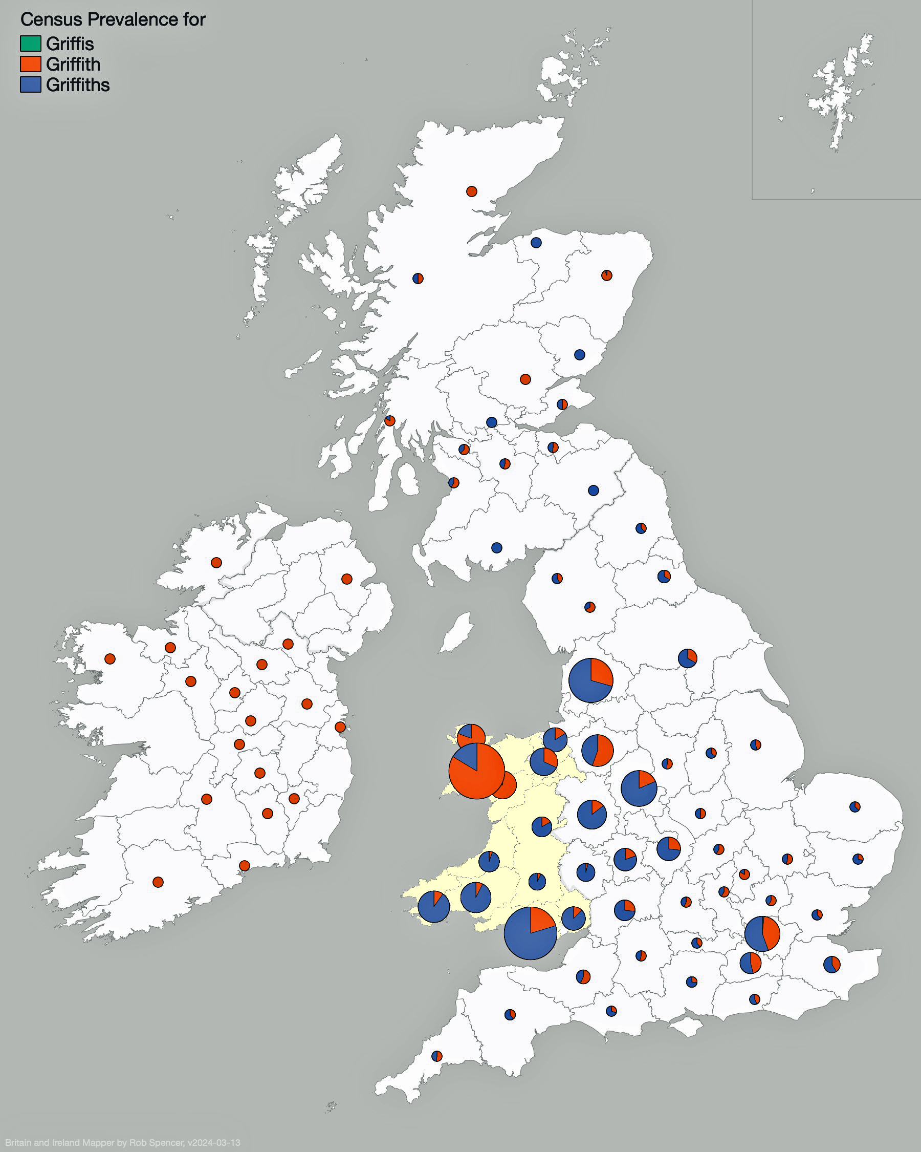
The following information was obtained from the innovative research strategies and tools of Rob Spencer, whose main interests are the exploration of genetic genealogy and population genetics. Rob Spencer’s Britain and Ireland SNP and Surname Mapper is a genealogical mapping tool that combines Y-DNA haplogroup analysis with 19th-century census data to visualize surname distributions and genetic ancestry across Britain and Ireland.
The tool is especially valuable for genealogists and researchers trying to trace Scottish, Irish, English, or Welsh paternal ancestry through a combination of genetic and historical data. The Mapper is particularly useful for identifying patrilineal origins when multiple surnames share common Y ancestry.
Looking at data for the ‘Griffis’ and Griffith’ surname distribution on map three, one can see that households with the Griffiths and Griffith surnames are located throughout Wales. Where the two surnames are relatively larger in specific counties, a small pie chart appears in Spencer’s Surname Mapperand portions of the pie reflecting areas proportionate to prevalence of the two surnames. Counties that have a lessor presence of the surnames are reflected with small dots. The Griffith and Griffiths surnames were present in small varying degrees in many of the counties of Great Britain and Ireland.
Map Three: Census Prevalence of Griffith & Griffiths Surnames in England and Ireland, Mid to late 1800s
The results of my traditional research of Welsh surnames indicate that there is compelling evidence that the Griff(is)(ith)(es) family line lived in the southern coastal region of Wales. There was also a strong possibility that ancestors related to the Griffis(ith(iths) family used other surnames such as Roberts, Owen, Owens, Williams and Hughes.
Using Genetic Genealogical Methods and Evidence: The Origin of the Patrilineal Family Line
The lack of tangible leads through traditional genealogical research sources and the advances of commercial direct-to-consumer DNA genealogical tests lead me to looking into Y-DNA genetic tests as a possible avenue to gain insights and possible leads on identifying information about the Griff(is)(ith)(iths)(es) line of descendants. [29]
See the following stories for genetic research on the Griffis family:
- Y-DNA & the Griffis Paternal Line Part Five: Using Y-DNA & Locating a Griff(is)(es)(ith) Relative and Other Leads March 3, 2023
- Y-DNA and the Griffis Paternal Line Part Four: Teasing Out Genetic Distance & Possible Genetic Matches February 24, 2023
- Y-DNA and the Griffis Paternal Line Part Three: The One-Two Punch of Using SNPs and STRs February 23, 2023
- Y-DNA and the Griffis Paternal Line Part Two: Snips and Strings and Other Interesting Things February 6, 2023
- Y-DNA and the Griffis Paternal Line – Part One September 26, 2022
Based on the limitations and the realistic expectations of what Y-DNA tests can find [30], I completed a Y-700 DNA test. [31] I had a few expectations of what I might be able to find by taking a Y-700 DNA test. Based on my traditional genealogical research I knew the Griffis family line had three spellings of the surname (Griffis, Griffith, and Griffes) in America and the use of a surname In Wales could also reflect variable spellings.
Two kinds of mutations make Y DNA genealogically useful for looking at the question of migration of a patrilineal line. They are short tandem repeat markers (STRs) and single nucleotide polymorphisms (SNPs). Both have their unique advantages in tracing Y-DNA mutations. [32]
SNP mutations occur rarely and are more stable across generations. They represent single point mutations in DNA sequence and rarely mutate back to their original form. SNPs are more reliable for determining deep ancestral lineage and can provide a basis for tracking migration patterns of genetic groups. [33]
STRs mutate rapidly (approximately one mutation every 20 generations). STRs are useful for examining recent ancestry within hundreds of years. [33] The configuration of STR mutations varies between individuals, creating unique Y-DNA haplotypes or genetic groupings among individuals. [34]
As indicated in a prior story, [35] the “One-Two” punch of testing involves using SNPs to provide a general location of Y-DNA testers on the Y-DNA haplotree based on nested haplogroups. Then, ‘the second punch’ uses Y-STR test results to group test results within recent haplogroup branches and assist in analyzing potential individual matches. The analysis and comparison of individual Y-STR haplotypes can help delineate lineages and tease out branches within the haplotree, fine-tuning relationships between people within the tree.
While STR tests are used by individual testers to discover possible Y-DNA genetic matches with other testers, the results of STR tests can also provide insights into macroscopic demographic properties that can shed light on lineages and clans – well before the time of surnames. Y- STRs have a time window that runs back to the late Bronze Age.
“STRs … tell us about demography — specifically about bottlenecks and subsequent expansions, namely “founder events.” While SNPs tell us when they were created, STRs tell us about when the population burgeoned after a founding mutation. That SNP and STR clades have a fundamentally different interpretation has caused considerable confusion, but once understood, the methods are very useful complements.” [36]
For genealogy within the most recent fifteen to twenty generations (about 500 to 660 years ago), STR markers help define paternal lineages and patterns around the advent of the use of surnames. STR analysis is an excellent approach to document genetic lineages before the use of surnames and into a period in which surname of genetically matched test kits could be different. For patrilineal lines a descent with Welsh surnames, this is important. The likelihood of finding genetic matches with test kits associated with different surnames is highly likely! [37]
I have used a number of Y-SNP and Y-STR tools and reports to help with my process of discovery. In addition to the FamilyTreeDNA reports, I have used tools created by individual genealogists that provide creative renditions of the data. For example, assuming there are sufficient testers to compare STR results, mutation history trees and dendrograms can be created illustrate genetic distance and graphically reveal genetic branches from hundreds of years back to the recent past ( fine-tuning the smaller branches, ‘twigs’, in a genetic tree). The STR tools are highly effective if used in tandem with SNP data and traditional genealogical information). [38]
Genetic Proof of Griffi(s)(th)(es) Family Paternal Line in Wales Through the Analysis of Y-DNA SNPs
The use of SNPs are a fairly straightforward process of figuring out where a male lands on a current or possibly new branch of the Y-DNA haplotree. The results of SNP tests are intuitive and easy in analyzing a group of other Y-DNA testers because they uniquely identify the haplogroup branches of descent. You can group testers in branches of a haplotree depending on whether their tests confirm or predict specific SNP mutations that represent specific branches of the haplotree. The Y-DNA haplotree allows individuals to trace their paternal ancestry and understand their place in human genetic history. [39]
The results of my Y-DNA analysis indicate the Griffis paternal line is part of a particular Y-DNA genetic branch that is not common among contemporary males in Europe. We are a minority genetically speaking and reflect the vestiges of a once dominant Y-DNA group.
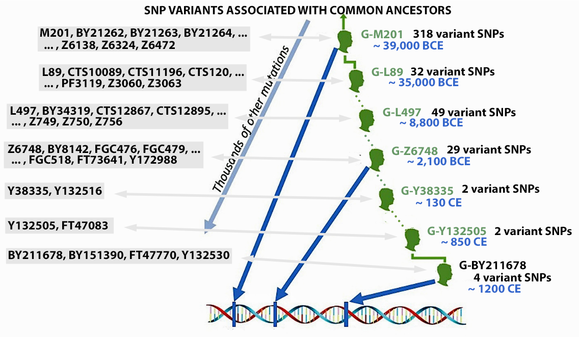
Illustration three provides an example of some of the major branches or subclades (SNP mutations ) of the G haplogroup of which the Y-DNA of Griff(is)(es)(ith) family can be traced. The illustration also indicates the sampled number of variant or equivalent SNPS associated with a particular branch. [40] Illustration three also indicates the approximate date of when the branch occurred (e.g. when a male exhibited a specific the SNP mutation).
Illustration Three: SNP mutations and the Patrilineal Line for Griffis Family
The Griff(is)(ith)(es) patrilineal line is part of the G Haplogroup and part of a major subbranch – the G2a-Haplogroup. A distinctive quality of the G2a-Haplogroup is it now appears at low frequencies across most of Europe, typically between one to ten percent of male lineages, with some notable exceptions. Higher concentrations are found in specific mountainous and isolated regions in Europe. [41]
Haplogroup G was associated with the spread of agriculture in Europe. It originated in West Asia and entered Europe during the Neolithic period. The highest genetic diversity of haplogroup G is in the northern Fertile Crescent, which suggests that this is where it originated. At one point it was the predominant haplogroup in Europe. While the G2a subbranch was once dominant among early European farmers, subsequent migrations and demographic changes have significantly altered its distribution. [42]
My Y-DNA test results indicate my terminal SNP value reflects a branch in the G Haplgroup that was located in an area that we now call Wales. A terminal SNP is the defining SNP (Single Nucleotide Polymorphism) that marks my placement on the most recent known branch of the Y-DNA haplotree. It represents the furthest down the tree branch where a positive result is obtained. [43]
Illustration three depicts the SNP Y-DNA mutation lines of descent from the Haplogroup G-L497 branch of the G-haplogroup to my terminal SNP branch. The illustration indicates the approximate dates of the Most Recent Common Ancestor (tMRCA) associated with each of these specific SNP branches. By viewing the approximate dates of each of the MRCAs for each of the branches, we can vaguely estimate when a Y-DNA ancestor possibly crossed from the European continent to the British Isles.
Illustration Three: Estimating When tMRCA Crossed the English Channel

My ‘terminal STR’ has been labeled as BY211678 or by FamilyTreeDNA as G-FT40897. [44] As reflected in the following chart, based on tracing the past sequence of SNP mutations, my common Y-DNA ancestors came to the English Isles about 1,050 years before the present. [45]
Chart One: Branches of the G Haplogroup from the G-FGC477 Sub-branch or Subclade
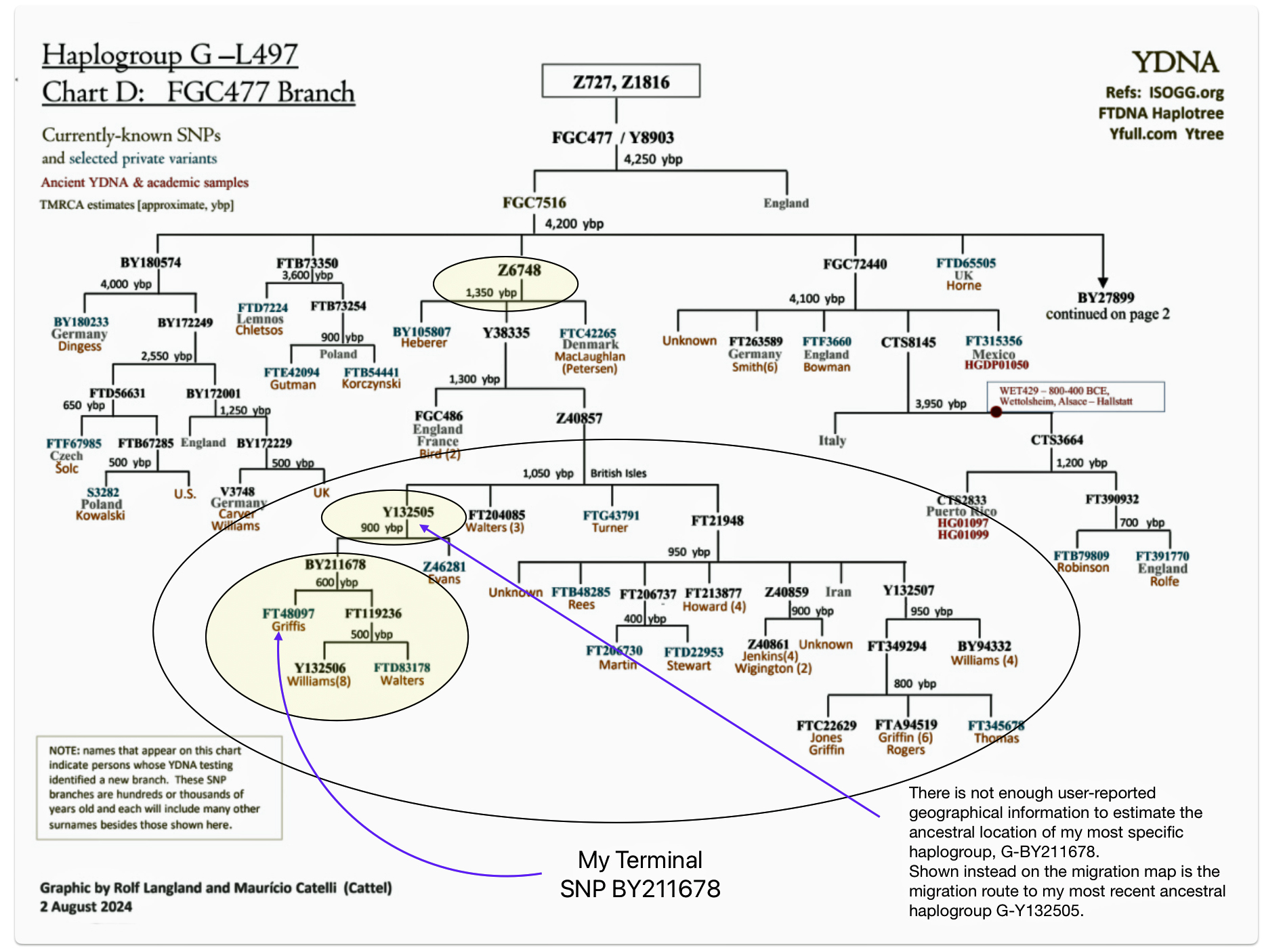
The large encircled area on the above graph represents G – haplogroup branches of Y-700 DNA test results that represent individuals whose ancestors inhabited the contemporary area of Great Britain. Their test results, including mine, can be traced to the most recent common ancestor (tMRCA) that lived around 1300 years before present (ybp). The yellow encircled branch that identifies the Y132505 subclade iis identified because it is the end point in map four below. The third yellow circle shows where my results reside in the context of common ancestors that branch off about 600 years ago – note the different surnames: Williams and Walters.
The following map four is a graphic portrayal of the migratory path of my Y-DNA genetic lineage produced through Globetrekker. Globetrekker is a mapping feature from FamilyTreeDNA for Big Y DNA test customers that traces paternal ancestral migration paths from Y-Adam in Africa (approximately 200,000 years ago) to recent times. The tool combines genetic data with geographical and historical information to map likely migration routes.
The map is generated through the use of software, that estimates geographical ancestor locations and migrations across the world based on the largest database of high-coverage Y-DNA sequences, ancient DNA results from archaeological remains, and user-reported ancestral locations. These are best estimates and will change over time as more people test their Y-DNA and provide information about their paternal line ancestry. [46]
Map Four: The Ancestral Migratory Path of the Griff(is)(ith)(es) Patrilineal Genetic Line
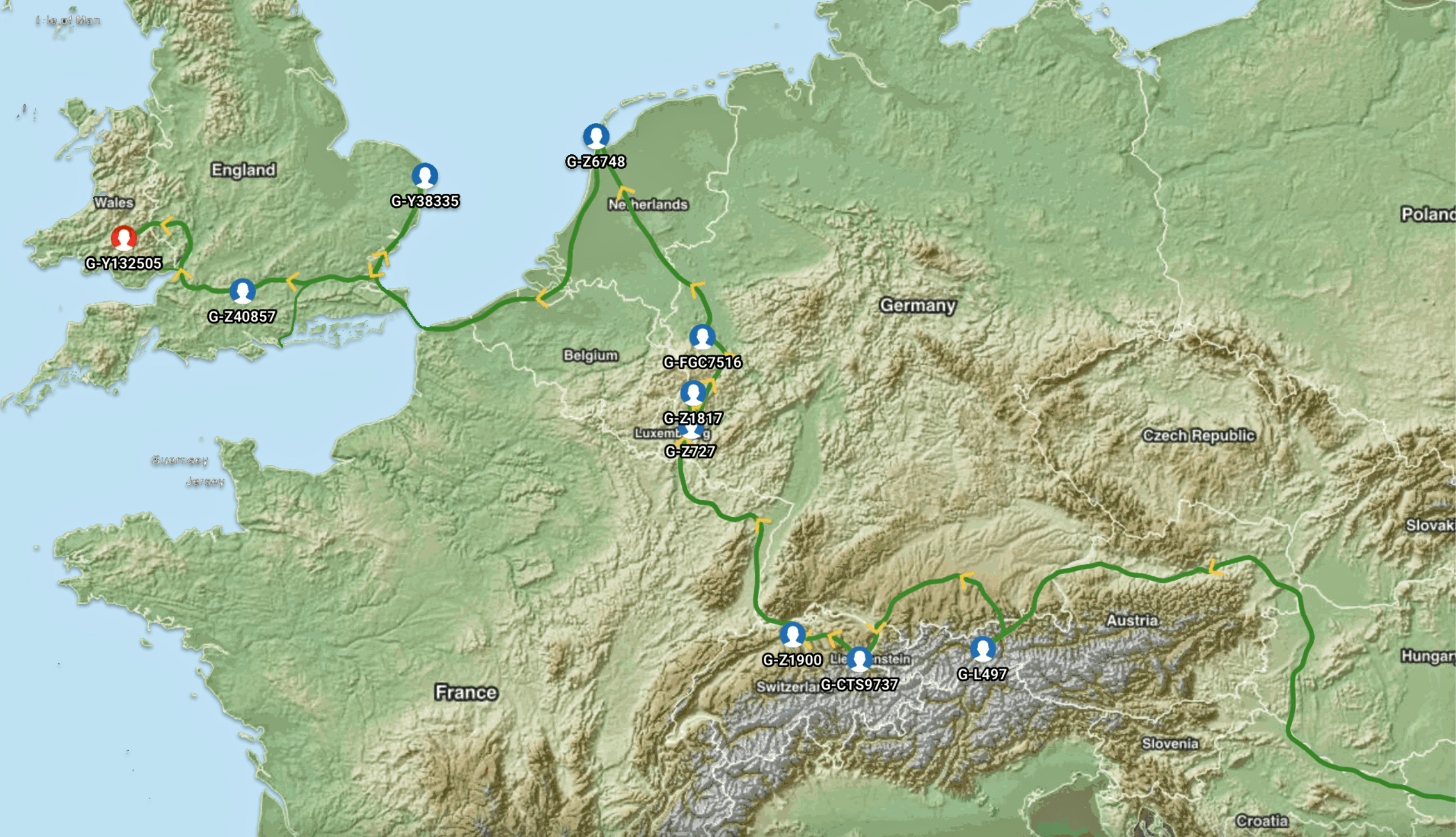
The general time periods associated with each of the subclades or the Most Recent Common Ancestors (tMRCAs) identified in the map are provided below. The end point of the migration follows subclade G-Y132505 which was referenced in chart one above.
Illustration Four: General Timelines Associated with tMRCAs
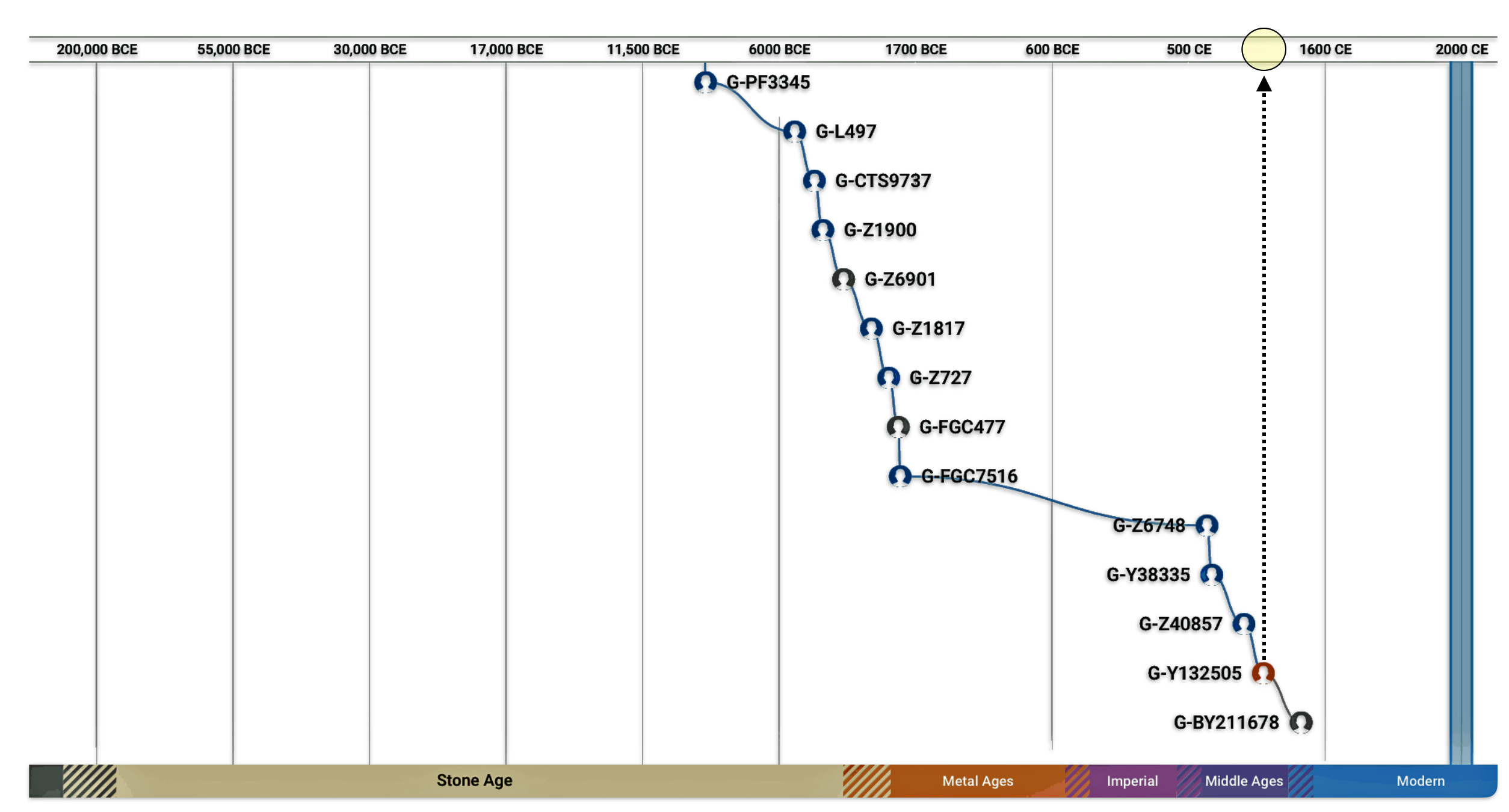
The map and related time frames associated with the Haplogroup subclades associated with my genetic lineage indicate ancestors of the family patrilineal genetic line came to the English Isles around 1000 CE and eventually inhabited an area that is now known as Wales. The analysis of SNP variants associated with my Y-700 DA test results provide strong evidence that my ancestors associated with my patrilineal line of descent lived in the geographical area that is Wales for about 500-600 years prior to the migration to the American Colonies.
A Welsh Connection Through the Analysis of Y-DNA STRs
There are a few STR markers that suggest the Griff(is)es)(ith) genetic line is Welsh. Haplogroup G-P303 (G2a2b2a) is a branch of haplogroup G (M201) that is a few branches pror to the G-L497 branch. This older haplogroup represents the majority of haplogroup G men in most areas of Europe west of Russia and the Black Sea. There are also some short tandem repeat (STR) findings among G-P303 men which help in subgrouping them.
The percentage of haplogroup G among available samples from Wales is overwhelmingly G-P303. Such a high percentage is not found in nearby England, Scotland or Ireland. The STR Marker DYS594=12 subgroup has an unusually high percentage of Welsh surnames with the rest mostly of English ancestry based on available samples. (Red highlighted in Table Three). [47]
Many of the men have an unusual value of 13 for Y-STR marker DYS388 ( I also have a 13 value for this marker which is yellow highlighted in Table Three), and some also have 9 at DYS568 (my value is 11). STR marker oddities are often different in each G-P303 subgroup, and characteristic marker values can vary by subgroup. Often the values of STR markers DYS391, DYS392 and DYS393, are respectively 10, 11 and 14 or some slight variation on these for all G-P303 men (all of these values of these markers I also have which are highlighted in blue in Table Three). [48]
In addition the DYS594 STR marker + 12 is a subgroup that has an unusually high percentage of Welsh surnames and to a lesser number of English ancestry. My value for this marker is 11.
Table 3 : FTDNA Y-111 STR Test Results for James Griffis – Markers 1 – 60

Another piece of evidence which supports the link between the surname and Wales is evidence I obtained from work with a FamilyTreeDNA working work, G-Z6748. Through initial research, the G-Z6748 appears to be a largely Welsh haplogroup.
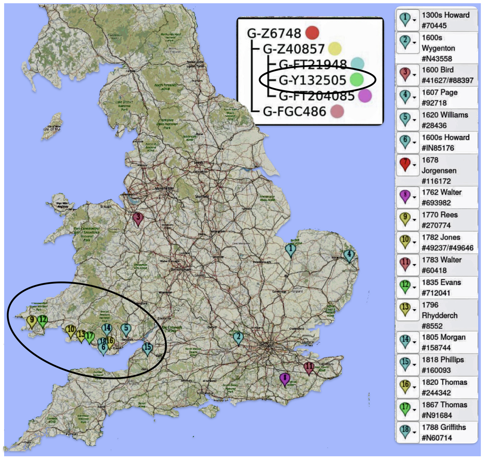
The Project Administrator of the group produced an interesting map that shows all known Z6748+ participants (and Y-Matches) who have traced their ancestor to a specific town in Wales. As can be seen below in map five, the majority of the group are tracing their ancestors to coastal southern Wales.
Map Five: Locations of Ancestor Origins of Z6748 DNA Testers
A third piece of evidence comes from the analysis of STR clusters between Y-DNA test kits within the Z6748 G subclade. The following Dendrogram [49] is from my analysis of test kits from the G-Z6748 Haplogroup Project. The dendrogram is the result of utilzing an innovative online program created by Rob Spencer that creates a graphic portrayal of data from FamilyTreeDNA. [50]
The dendrogram is similar to a family tree. The individual DNA testers are the dots at the right of the diagram. On a traditional family tree, branch points are ancestors. On the dendrogram branch points are not people but points in time when genetic changes occurred.
Time moves backward to the left. Time is measured in generations which roughly equates to 31 years per generation. I have added how many years before present (ybp) and the approximate year each given generation mark represents. Each Line represents a Y-DNA test kit. The defined haplogroup for each test kit is listed. Depending on the type of D-DNA test completed, some of the haplogroups are very detailed while others are very general. The name of the paternal ancestor that was provided by each individual who completed the Y-DNA test is also listed.. I have also highlighted an area that depicts the range of time where the use of surnames became part of family tradition.
Illustration Five: Dendrogram of Y-DNA Test Kits in the Z6748 Subclade
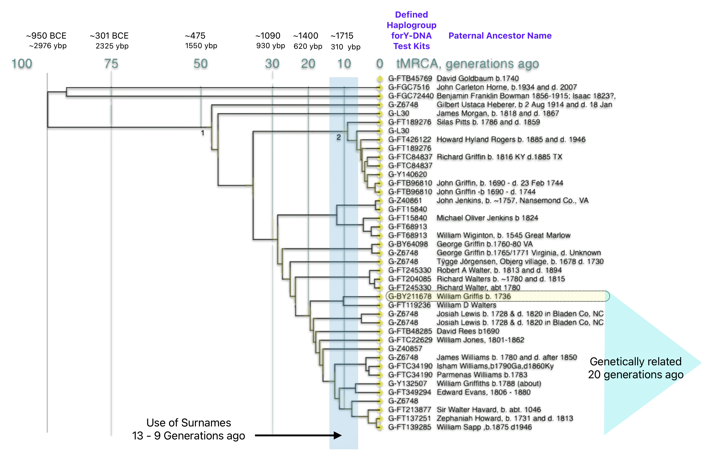
The dendrogram graphically reflects the genetic closeness of test kit results that share Y-DNA mutations within the G-Z6748 branch. The Dendrogram shows my test kit (that is highlighted in yellow) and my geneetic relationship with the other test kits. I share a common paternal genetic ancestor with a test kit that has an ancestor named William D. Walters. Our common ancestor lived about 10 generations ago or about 300 years ago – before William’s ancestors immigrated to the colonies. I also share common genetic paternal ancestors with 14 other test kits with a most recent common ancestor that lived around 20 generations ago or about 600 years ago. What is noteworthy with these common paternal genetic ties is the variability of surnames: Walters, Lewis, Rees, Jones, Howard, Harvard and Sapp.
The Use of Research Standards and Methods from Different Disciplines
“All genealogists strive to reconstruct family histories or achieve genealogical goals that reflect historical reality as closely as possible.” [51] This general goal and standard requires the adherence to and application of standards for conducting sound, reliable research and utilizing various research methods to obtain and analyze facts and evidence.
“Crisis being the twin of opportunity, the field (of genealogy) has accepted the challenge of educating such massive numbers outside any institutional system of education. That exigency has generated a scrutiny of almost all precepts by which families are studied and evidence is analyzed—much of that effort being made by the Board for Certification of Genealogists. The result has been another marked advance in the maturity of the field, beginning with an increased emphasis upon documentation, methodology, and record interpretation—and drawn from the interdisciplinary study of economics, genetics, geography, law, medicine, military and monetary systems, politics, and psychology, as well as all aspects of history.” [52]
For me, similar to Elizabeth Mills’ statement above, these ‘standards’ for conducting research and the ‘various methods’ for analyzing genealogical facts and evidence come from various disciplines. In addition to genealogical standards and methods, various fields of social and historical research and journalism have standards and approaches that have influenced my approach in conducting genealogical research.
Each discipline has their unique view and advantages. The standards for various professional organizations essentially require exhaustive research, citation and documentation of sources, analysis and correlation of data, resolution of conflicting evidence, and soundly written conclusions.
My formal research training was in the social sciences. I have acquired a formal and practical understanding and application of various approaches for collecting and analyzing facts and evidence. I have an understanding of how to use various qualitative and quantitative research methodologies to analyze genealogical facts and evidence. [53]
I have also been influenced by social historians that have employed innovative methods that characterized the “new social history” approach that emerged during in the 1970s. Social historians shifted away from studying “great men” and larger historical forces to examine the lives and experiences of ordinary people. This “history from below” approach aimed to reconstruct the perspectives of common people throughout history. [54] Social Historians and professional Genealogists have increasingly documented the benefits of genealogy as a source of historical information and research methods associated with records and archival-research skills. [55]
While my goal is not to obtain professional credentials in the area of genealogical research, I share and utilize many of the standards espoused by organizations that are associated with genealogical research. There are two main organizations in the United States that award credentials to professional genealogists: the International Commission for the Accreditation of Professional Genealogists (ICAPGen℠) and The Board of Certification for Genealogists (BCG). While both credentials demonstrate a high level of genealogical research ability, there are some key differences between the two programs. [56]
Development of Genealogical Standards
Genealogical organizations developed research standards over the last century to improve the quality, reliability, and credibility of genealogical research. As genealogy transitioned from a niche hobby to a massive popular pursuit over the last century, major genealogical organizations developed research standards to maintain ‘rigor and credibility’. [57]
Several key factors drove this evolution.
Increasing Popularity and Accessibility of Genealogy: As interest in genealogy exploded in the 20th century, fueled by more available books, records, and later the Internet, genealogical organizations saw a need for standards to guide the growing ranks of both professional and amateur researchers. Standards would help genealogists, regardless of background, “get their genealogy right” and avoid inaccuracies and myths. [58]
Need for More Rigorous Proof Standards: Genealogists initially borrowed the legal principle of “preponderance of evidence” to justify conclusions. However, it became clear that simply having more evidence for a conclusion was not sufficient for sound genealogical proof. More analysis of the quality of sources and information and resolution of conflicts was needed. Prominent genealogists pushed for “convincing arguments and clearly stated conclusions, including reasoned explanations of any conflicting evidence”. [59]
Cover of American Genealogist
Drive to Improve Genealogy’s Scholarly Reputation: Scholarly genealogy journals in the late 20th century began expecting research articles to demonstrate high standards of evidence and reasoning. Genealogical organizations like the Board for Certification of Genealogists took the lead in defining research standards, publishing the first Genealogical Standards Manual in 2000. The goal was to establish genealogy as a rigorous field of historical research. [60]
Advent of Technology and Big Genealogy Databases: The rise of computerized genealogy databases and Internet genealogy companies in recent decades made standards even more crucial. Genealogists needed to understand the coverage and limitations of these massive but incomplete data sources. Standards provided a basis for evaluating the reliability of database information and online trees. [61]
Current Genealogy Standards
Major genealogical organizations have established research and ethical standards to promote accuracy and credibility in the field. By documenting sources well, sound reasoning, and acknowledging the limits of evidence, genealogists can produce more reliable family histories. [62]
For example: the Board for Certification of Genealogists (BCG) has published “Genealogy Standards” detailing standards for documenting, researching, and writing family histories. The National Genealogical Society (NGS) has also published “Standards for Sound Genealogical Research” outlining best practices.
These standards cover issues like thoroughly documenting sources, analyzing and correlating evidence, resolving conflicts, and accurately reporting findings. They aim to uphold the integrity of the field.
Some of the notable objectives are:
Original Records and Proper Documentation: Genealogical standards emphasize using original records whenever possible, rather than relying solely on compiled works or online trees. Genealogists are expected to document their sources thoroughly so others can evaluate the evidence.
Transparency and Openness: Standards encourage genealogists to make their research transparent, sharing their sources, analysis, and reasoning. This allows the genealogical community to scrutinize conclusions and keeps researchers accountable.
Citing Sources in Compiled Works: When publishing family histories, genealogists should cite their sources using standard citation formats. Endnotes or footnotes are preferred over simply listing sources at the end. This allows readers to easily connect specific facts to the evidence supporting them.
Separating Facts from Hypotheses: Genealogical writing standards call for clearly distinguishing proven facts from theories or possibilities. Genealogists should explain their reasoning and acknowledge the limits of indirect evidence.
Parting Words
Genealogical research prior to the technological advances of the internet and the increased accessibility of historical data faced several significant challenges despite growing popularity during this period. Research required extensive travel to private and governmental repositories, government county clerks offices, and libraries and archives. Not only was it often cost-prohibitive to travel, the ability to access and transcribe information was challenging and time consuming. Geographic and political boundaries frequently prevented access to crucial records. Researchers had to rely primarily on family oral history and family documents, vital records, city/county directories, church and cemetery records, local newspapers and periodicals.
“In the 20th century, most genealogists conducted their research by interviewing relatives and visiting repositories to inquire about their ancestors. Travel to these sites was almost a necessity, but genealogists were often hindered by the geographic (and sometimes political) boundaries in which they lived. Travel out of their region was also cost prohibitive. When they could access original documents, they relied on vital records, city/county directories, and church/cemetery records to reveal new information or provide a clue to a new individual or branch of their family tree. Old newspapers and periodicals could also reveal the socio-economic reasons of an era for migration to, and around, the United States. Additionally, books and journals would inform a genealogist on how to research their roots and organize the data.” [63]
Primary source documents were difficult to access as they were not originally created for genealogical purposes and often lacked proper indexing or organization. Census records had strict access restrictions, requiring approved researchers to conduct their work at National Archives facilities with limited reproduction permissions. [64]
Only wealthy and noble families traditionally maintained detailed documentation of their ancestry. Record-keeping was inconsistent, and many documents were scattered across multiple locations and not properly indexed or organized [65]
Genealogists faced barriers in technically accessing historical records. Record linkage between censuses was extremely labor-intensive, with researchers having to manually search through microfilmed listings. The Soundex indexing system, while helpful, was organized state-by-state on microfilm, making interstate migrant searches expensive and often unsuccessful. Success rates for tracking individuals between censuses (known as “persisters”) were typically under 40 percent. [66]
The field of genealogy faced skepticism from academic historians, who did not view genealogists as serious researchers until the rise of social history in the late 1960s. This attitude began to shift as social history topics gained popularity, leading to increased interest in genealogical research methods. [67]
The research process was extremely time-consuming. It involved writing and receiving letters from county clerks and other officials if one were limited by travel. A lot of time was spent on manual searching through unindexed records. Typing family histories on typewriters with frequent corrections was the norm. This methodical pace, however, had one advantage – researchers spent more time analyzing each record and understanding its context within the broader historical picture. [68]
The advent of accessible, digital records on the internet, the commercialization of genealogical research data, and the introduction of search capabilities of the digital data have made it much easier to research large amounts of evidence and document our genealogical discoveries.
“In this age of all these emerging technologies, genealogists’ information seeking behaviors and needs are evolving and adapting at a greater speed than ever before. Genealogists can locate information relevant to their family search with just a few clicks on a website. They can download and/or purchase digital images of documents such as birth records, cemetery records, and census records. The number of online resources can be overwhelming, and care must be taken to ensure the provenance and authenticity of the information they discover.” [69]
While it is easier to find data and evidence, the tedious and hard work associated with critically analyzing all the available data and evidence does not become easier. Research and analysis of evidence becomes more challenging. The results of our research, whether it is meticulous or casually produced, can have more pronounced impact since information travels more freely in the digital era.
This is why the use of genealogical research standards and the understanding of the benefits and limitations of various research methodologies and aproaches to gatehring and analyzing evidence is so important.
Sources
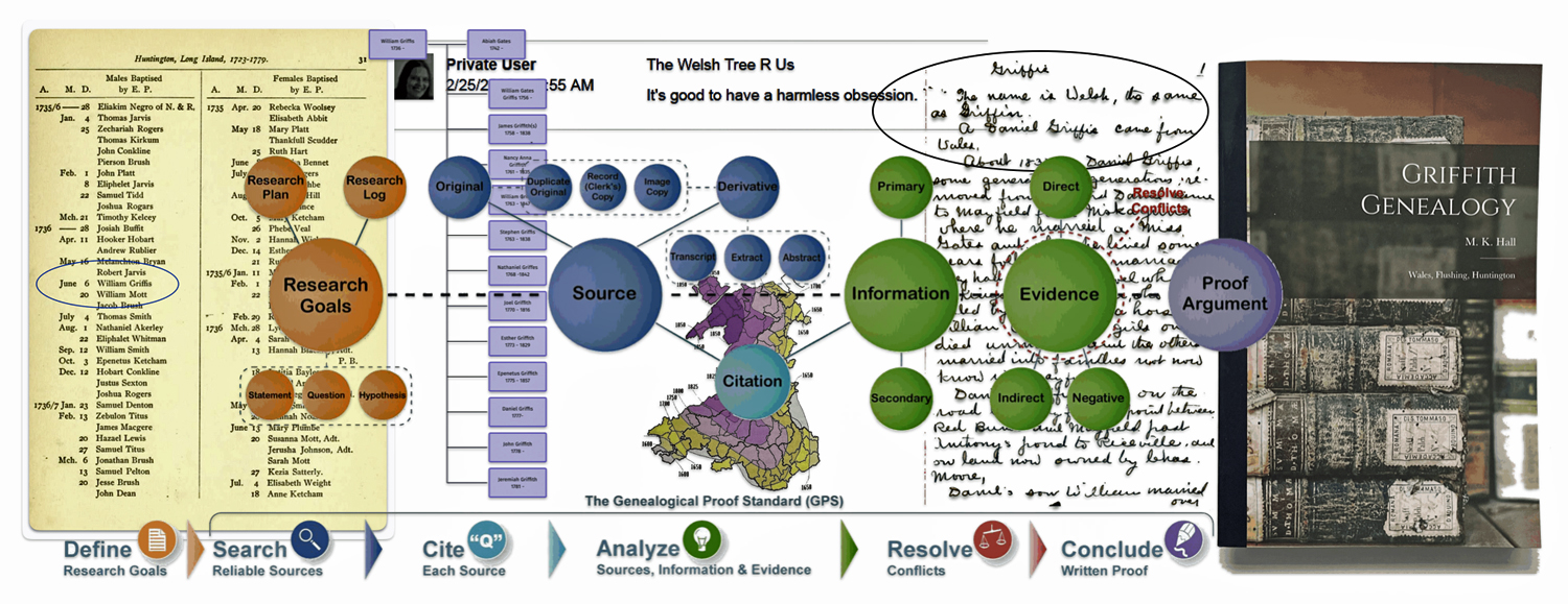
Feature Image: The map was created in 2008 by Mark Tucker as a visualization of the genealogy research process. It is meant as a tool for genealogists and family historians from beginner to professional. It combines concepts from the Board for Certification of Genealogists and the works of professional genealogist, Elizabeth Shown Mills. https://www.familysearch.org/en/wiki/Genealogy_Research_Process_Map
Behind the diagram of the genealogy research process are examples of evidence used in the story..
[1] For additional reading on this subject, see the following references:
Gregory Rodriguez, How Genealogy Became Almost as Popular as Porn, May 30, 2014, Time, https://time.com/133811/how-genealogy-became-almost-as-popular-as-porn/#
Maya Jasanoff, Our Obsession with Ancestry Has Some Twisted Roots, The New Yorker, May 2, 2022, https://www.newyorker.com/magazine/2022/05/09/our-obsession-with-ancestry-has-some-twisted-roots-maud-newton-ancestor-trouble
Rebecca Dalzell, Genealogy: the Second Most Popular Hobby in the US?, April 27, 2017, Ancestry.com Blog, https://blogs.ancestry.com/cm/genealogy-second-most-popular-hobby-us/
Maud Newtown, America’s Ancestry Craze, Harpers, https://harpers.org/archive/2014/06/americas-ancestry-craze/
[2] Andy Lee, Family Fanatics History, Blog, https://www.familyhistoryfanatics.com/genealogy-isnt-that-popular
James Tanner, Hobby Claims about Genealogy are Unfounded, June 4, 2014, Genealology’s Star, Blog, https://genealogysstar.blogspot.com/2015/06/hobby-claims-about-genealogy-are.html
James Tanner, Is Genealogy a hobby or pastime?, 10, 2016, LDS Blogs, https://rejoiceandbeexceedingglad.blogspot.com/2016/11/is-genealogy-hobby-or-pastime.html
How Popular is Genealogy?, Genealogy inTime Magazine, Blog, Page accessed on Jan 7, 2024, http://www.genealogyintime.com/articles/how-popular-is-genealogy-page01.html
Genealogy is NOT the Second Most Popular Hobby in the US https://www.familyhistoryfanatics.com/genealogy-isnt-that-popular
Is Genealogy Growing? http://www.genealogyintime.com/articles/how-popular-is-genealogy-page06.html
Genealogy: the Second Most Popular Hobby in the US? https://blogs.ancestry.com/cm/genealogy-second-most-popular-hobby-us/
Hobby Claims about Genealogy are Unfounded https://genealogysstar.blogspot.com/2015/06/hobby-claims-about-genealogy-are.html
[3] Hjorthén Adam , Reframing the History of American Genealogy: On the Paradigm of Democratization and the Capitalization of Longing. Genealogy. 2022; 6(1):21. https://doi.org/10.3390/genealogy6010021
[4] Jackson, Chris, Majority of Americans think knowing their ancestry is important, 25 Jun 2021, IPSOS, https://www.ipsos.com/en-us/majority-americans-think-knowing-their-ancestry-important
[5] Scholars have written about the “democratization of genealogical research” (Lenstra 2015, p. 203), a “democratize[d] access to the past” (De Groot 2015, p. 119), “a democratization of sources” for genealogical research (Tucker 2016, p. 165), “a democratic and expanded notion of relatedness” (Creet 2020, p. 168), a “democratic interest in family history” (Weil 2013, p. 181), and “the development of public interest in genealogy could be highlighted as popular, and democratic” (Hering 2009, p. 5)
De Groot, Jerome. 2015. On Genealogy. The Public Historian 37: 102–27.
Tucker, Susan. 2016. City of Remembering: A History of Genealogy in New Orleans. Jackson: University Press of Mississippi.
Creet, Julia. 2020. The Genealogical Sublime. Amherst: University of Massachusetts Press.
Weil, François. 2013. Family Trees: A History of Genealogy in America. Cambridge: Harvard University Press.
Hering, Katharina. 2009. “We Are All Makers of History”: People and Publics in the Practice of Pennsylvania-German Family History, 1891–1966. Ph.D. thesis, George Mason University, Fairfax, VA, USA.
See other writings for example:
Lenstra, Noah , ‘Democratizing ‘ Genealogy and Family Heritage Practices: theView from Urbana, Illinois, In Encounters wth Popular Pasts: Cultural Heritage and Popular Culture, Mike Robinson and Helaine Silverman, eds., NewYork: Springer 2015, Page 203
De Groot, Jerome, On Genealogy, The Public Historian, Volume 37, Issue 3, August 2015, Page 119, https://online.ucpress.edu/tph/article-abstract/37/3/102/89479/International-Federation-for-Public-History?redirectedFrom=fulltext
Tucker, Susan. 2016. City of Remembering: A History of Genealogy in New Orleans. Jackson: University Press of Mississippi, 2016, Page 165
Creet, Julia, The Genealogical Sublime, Amherst: University of Massachusetts Press, 2020, Page 168
Weil, François. 2007. John Farmer and the Making of American Genealogy. New England Quarterly 80. Pages 408–34., Page 181, https://direct.mit.edu/tneq/article-abstract/80/3/408/15801/John-Farmer-and-the-Making-of-American-Genealogy?redirectedFrom=fulltext
Hareven, Tamara, K., The Search for Generational Memoriy: Tribal Rites in Industrial Society. Daedalus, 107, 1978, Pages 137 – 149
Taylor, Robert M. 1982. Summoning the Wandering Tribes: Genealogy and Family Reunions in American History. Journal of Social History 16, Pages 21–35, https://academic.oup.com/jsh/article-abstract/16/2/21/1031592?redirectedFrom=fulltext
Bidlack, Russell E. 1983. Librarians and Genealogical Research. In Ethnic Genealogy: A Research Guide. Edited by Jessie Carney Smith, Westport: Greenwood Press.1983, Page 9
Morgan, Francesca. 2010a. A Noble Pursuit? Bourgeois America’s Uses of Lineage. In The American Bourgeoisie: Distinction and Identity in the Nineteenth Century. Edited by Sven Beckert and Julia Rosenbaum. New York: Palgrave, 2010
[6] I have provided four PDFs of the entire discussion thread since, as the last comment declares, “wow what an….. interesting discussion I’ve stumbled upon“.
PDF One | PDF Two | PDF Three |PDF Four
John Stephen Saponaro, Discussion Thread on John ap Gruffudd (Pengruffwnd) – Wales in April 2020, Gene Collaboration Website, Thread started 14 Feb 2020. Discussion Thread accessed 7 Jan 2022. https://www.geni.com/discussions/208254
Ann Brannen, Discussion Thread on John ap Gruffudd (Pengruffwnd) – Wales in April 2020, Gene Collaboration Website, Thread started 14 Feb 2020. Page 2 of the discussion Ms. Brannen’s post was on 25 Feb 2020 7:55 am, Discussion Thread accessed 7 Jan 2022.
[7] O’Hare, Sheila, Genealogy and History, April 2002, Common Place, https://commonplace.online/article/genealogy-and-history/
[8] Adam Hjorthén, Genealogy from a distance: the media of correspondence and the Mormon church, 1910–45, Historical Research, Volume 94, Issue 263, February 2021, Pages 117–135, https://doi.org/10.1093/hisres/htaa034
[9] Elizabeth Shown Mills, Working with Historical Evidence: Genealogical Principles and Standards, Vol 87, No. 3, Sep 1999, Evidence, A special Issue of the National Genealogical Society Quarterly, Pages 169, https://www.historicpathways.com/download/workwthhistevidence.pdf.
[10] See my story: Griffis, Jim, Griff(is)(in)(ith)(iths)(es)(in)(ins)(ing) Surname and American Genealogies: Part One, Feb 17, 2022, Griffis Family: Selected Stories from the Past, https://griffis.org/griffisinththsesininsing-surname-and-american-genealogies-part-one/
[11] Griffith, Laura, The Griffith’s of Wales and America, Self published Mayfield, KY: 1979, reprinted 1982. Page IV,
[12] The Genealogical Proof Standard – International Institute, FamilySearch Wiki, This page was last edited on 27 April 2023, https://www.familysearch.org/en/wiki/The_Genealogical_Proof_Standard_-_International_Institute
Morton, Sunny Jane, The Genealogical Proof Standard: An Expert Explanation for Guiding Your Research, FamilyTree, https://familytreemagazine.com/strategies/genealogical-proof-standard/
Chapter 1: The Genealogical Proof Standard, Family History and Genealogical Research, https://books.byui.edu/fhgen_110_textbook_/chapter_1__the_genealogical_proof_standard
[13] Genealogical Proof Standard, Wikipedia, This page was last edited on 11 November 2024 , https://en.wikipedia.org/wiki/Genealogical_Proof_Standard
Genealogical Proof Standard, FamilySearch Wiki, FamilySearch, This page was last edited on 30 April 2023, https://www.familysearch.org/en/wiki/Genealogical_Proof_Standard
McDermott, Marc, Genealogical Proof Standard, 12 Feb 201 8, updated 11 Oct 2024, GenealogyExplained, https://www.genealogyexplained.com/basics/genealogical-proof-standard/
Stahle, Tyler, Understanding the Genealogical Proof Standard, 9 Mar 2016, FamilySearch Blog, https://www.familysearch.org/en/blog/understanding-the-genealogical-proof-standard
Understanding Genealogical Proof, National genealogical Society, https://www.ngsgenealogy.org/going-to-the-next-level/understanding-genealogical-proof/
[14] Zeno Griffin, Richard Pengruffwnd , New York Genealogical and Biographical Record vol. 37 , 1906. p. 54-55.
[15] Griffin, Paul, Annotated Bibliography of the Griffin/Griffen Family, Freepages Rootsweb.com, 27 Feb 1995, Revised Dec 1999, page accessed 6 Jun 2015. Paul Griffin provides an excellent bibliography of published and unpublished books, articles or manuscripts about Griffin(th)(ths)(is) families. His genealogical focus concerns the descendants of Edward Griffin purportedly born around 1602 in Wales and his siblings. For a PDF copy of the annotated bibliography click here.
Hugh Lavry, Edward Griffin (abt. 1602 – abt. 1706), WikiTree.com, Profile last modified 28 Aug 2020, Created 27 Jan 2011, Accessed 12 Dec 2021.
The Flushing Remonstrance, 1657, Historical Society of the new York Courts, Page accessed 05 Dec 2021
Kristina Wheeler, , Edward Griffin (abt. 1648 – abt. 1742), Wikitree.com, Profile last modified 12 Apr 2019, Created 27 Jan 2011, Accessed 12 Dec 2021.
Susannah (Griffin) Barnett (abt. 1662 – 1742), WikiTree.com, Profile last modified 19 Jun 2020, Created 27 Jan 2011, Accessed 12 Dec 2021.
Hugh Lavry, Richard Griffin (abt. 1670 – 1723), WikiTree.com, Profile last modified 24 Dec 2017, Created 27 Jan 2011, Accessed 12 Dec 2021.
John Thompson, Deborah Griffin (abt. 1662), Wikitree.com, Profile last modified 1 Jul 2020 | Created 27 Jan 2011, Page accessed 12 Dec 2021.
Theresa Griffin, Debunking the Published Griffin Family Myths: Edward Griffin of Flushing was not Edward Pengruffwnd (Pengriffin) of Walton West, Pembrokeshire, Wales, freepages.rootsweb.com, Page last edited September 2009, page accessed 9 Dec 2021. For a PDF version of the website citation, provided in the event the website version is discontinued.
Z T Griffen and Rev Duane N Griffin, Sgt. John Griffin of Simsbury Conn , The New York Genealogical and Biographical Record Vol XLIX No 1 , January 1918, Page 23-26
[16] Theresa Griffin, Debunking the Published Griffin Family Myths: Edward Griffin of Flushing was not Edward Pengruffwnd (Pengriffin) of Walton West, Pembrokeshire, Wales, freepages.rootsweb.com, Page last edited September 2009, page accessed 9 Dec 2021. For a PDF version of the website citation, provided in the event the website version is discontinued.
[17] Ibid
[18] The three manuscripts are:
The Peets-Griffith manuscript: Mildred Griffith Peets, Griffith Family History in Wales 1485–1635 in America from 1635 Giving Descendants of James Griffis (Griffith) b. 1758 in Huntington, Long Island, New York, compiled by Capitola Griffis Welch, 1972 . PDF copy of the manuscript can be found here.
The Jones-Welch manuscript: Mary Martha Ryan Jones and Capitola Griffis Welch, compiled by, Griffis Sr of Huntington Long Island and Fredericksburg, Canada 1763-1847 and William Griffis Jr, (Reverend William Griffis) 1797-1878 and his descendants. A self published genealogical manuscript, 1969. PDF copy of the manuscript can be found here.
The Hall manuscript: M.K. Hall, Griffith Genealogy: Wales, Flushing, Huntington, Unpublished Manuscript 1929, originally published 1937, https://archive.org/details/griffithgenealog00hall/page/n3/mode/2up
[19] See :
Welsh Surnames, Genealogy Today, Page accessed 1 November 2021.
John and Shiela Rowlands, The Surnames of Wales: For Family Historians and Others, Baltimore, MD: Genealogical Publishing Co. 1966
John and Shiela Rowlands, ed, Stages in Researching Welsh Ancestry. England: The Federation of Family History Societies Publications Ltd., 1999
John Davies; Nigel Jenkins; Menna Baines; Peredur I. Lynch, eds. (2008). The Welsh Academy Encyclopedia of Wales. Cardiff: University of Wales Press. p. 838.
Welsh Surnames, Wikipedia, Page edited 3 Oct 2021, page accessed 9 Dec 2021
Wales Personal Names, FamilySearch.org , this page was last edited on 17 August 2021, page was accessed 7 Jan 2022.
Craig L. Foster, Welsh Naming Patterns, FamilySearch.org, 2015, PDF accessed 12 Dec 2021
Ben Johnson, The History of Welsh Surnames, Historic UK: The History and Heritage Accommodation Guide, page accessed 11 Nov 2021
Welsh Surnames: Why are there so many Joneses in Wales?, Amgueddfa Cymru — National Museum Wales, page accessed 9 Sep 2021
Tamie Dehler, Before fixed surnames, Welsh followed a Celtic naming system, Tribunte-Star: Terre Haute and Wabash Valley, Nov 28, 2010 Updated Aug 6, 2014, page accessed 20 Nov, 2021
Donald Moore, The Indexing of Welsh Names, The Indexer, Volume 17, Number 1, April 1990, accessed 06 Apr 2020
Welsh Patronymics Group Project, FamilyTreeDNA
Rowlands, Shiela, The Surnames of Wales, Chapter 7, in John & Shiela Rolands, Welsh Family History: A Guide to Research, Second Edition, Baltimore: Genealogical Publishing Company, 1998, page 62
Shiela Rowlands, Sources of Surnames in John and Shiela Rowlands, ed, Stages in Researching Welsh Ancestry. Bury, England: The Federation of Family History Societies Publications Ltd., 1999. Pages 153 and 159
Durie, Bruce, Welsh Genealogy, Stroud, United Kingdom: The History Press, 2013, Page 27
John Rowlands, The Homes of Surnames in Wales, in John and Shiela Rowlands, ed, Stages in Researching Welsh Ancestry. Bury, England: The Federation of Family History Societies Publications Ltd., 1999. Page 162-164
John and Sheila Rowlands, The Use of Surnames, Chapter 4, Patronymic Naming – A survey in Transition, Llandysul, Ceredigion: Gomer Press, 2013, Pages 50-57
[20] Griffis, Jim, Part Three: How Do You Spell Griffis?, April 2, 2022, Griffis Family: Selected Stories from the Past , https://griffis.org/part-three-how-do-you-spell-griffis/
[21] 1799 New YorkTax Assessment Rolls of Real and Personal Estates, 1799 – 1804, Suffolk County, 1801, Huntington, Image 8, Lines 30, 31 and 37.
Data source: New York State Archives, Ancestry.com. New York, U.S., Tax Assessment Rolls of Real and Personal Estates, 1799-1804 [database on-line]. Provo, UT, USA: Ancestry.com Operations, Inc., 2014. Original data: New York (State), Comptroller’s Office. Tax Assessment Rolls of Real and Personal Estates, 1799–1804. Series B0950 (26 reels). Microfilm. New York State Archives, Albany, New York.
[22] Correlation tools verify the accuracy of information by comparing details across different sources and identifying consistent patterns to confirm family relationships.
Some of the common methods or tools are:
- Comparison tables: Creating tables to directly compare information like names, birth dates, marriage dates, and locations from multiple records side-by-side.
- Timelines: Visualizing events in chronological order to identify potential connections between individuals based on their life stages and locations.
- Maps: Using geographical information to pinpoint locations mentioned in records and see if they align with known family patterns.
- Cluster research: Identifying associated individuals (neighbors, friends) around a potential ancestor to gather more context and potentially uncover missing information.
“The problem is that in genealogy, we are not always handed a 100% match, there are discrepancies concerning a person’s facts in the sources we collect. Sometimes there are larger discrepancies, such as of three major pieces of information in a genealogical profile: names, dates, and location. Individuals may have used a certain alias or alternated one of their given names as their first name. Dates are even shakier because our ancestors may not correctly remember the birth date. They may also enact leniency on their true age, so they state they are younger than they actually are. Of these, the one part of our ancestor’s profile that is the most important is the location. Our ancestors could not clone themselves, so while they could change the facts about their life to assume a new identity, it’s very hard to discredit evidence concerning location.”
Fletcher, Jake, Is it a Match: Ways to Correlate Evidence and Identify Ancestors, 15 May 2016, Legacy Family Tree Software, https://legacyfamilytree.com/blog/2016/05/is-it-a-match-ways-to-correlate-evidence-and-identify-ancestors/
Jones, Thomas, Using “Correlation” to Reveal Facts that No Record States, 2012, FamilySearch, https://cms-b-assets.familysearch.org/4b/71/a2f6de0e0aa0b1347419c72020d7/course-handout.pdf
[23] The story is attributed to Albert Buffet Griffith (18 Sep 1826 Huntington NY – 24 Mar 1901 Huntington NY). His lineage in the Griffis(th) family reflects the changes in the spelling of the surname. His father was Peter Griffith (1792 Huntington NY – 1864 Huntington NY), his grandfather was James William Griffis (04 Jun 1758 Suffolk Co – 21 Nov 1838 Suffolk Co) and his great grandfather was William Griffis.
See: The Jones-Welch manuscript: Mary Martha Ryan Jones and Capitola Griffis Welch, compiled by, Griffis Sr of Huntington Long Island and Fredericksburg, Canada 1763-1847 and William Griffis Jr, (Reverend William Griffis) 1797-1878 and his descendants. A self published genealogical manuscript, 1969. PDF copy of the manuscript can be found here.
[24] Griffis, Jim, Recent Discoveries from Oral History Compiled by a Local Mayfield Historian – Part I, 28 Mar 2024, Griffis Family: Selected Stories from the Past, https://griffis.org/recent-discoveries-from-oral-history-compiled-by-a-local-mayfield-historian-part-i/
[25] The following is the first page Rulifson’s notes:
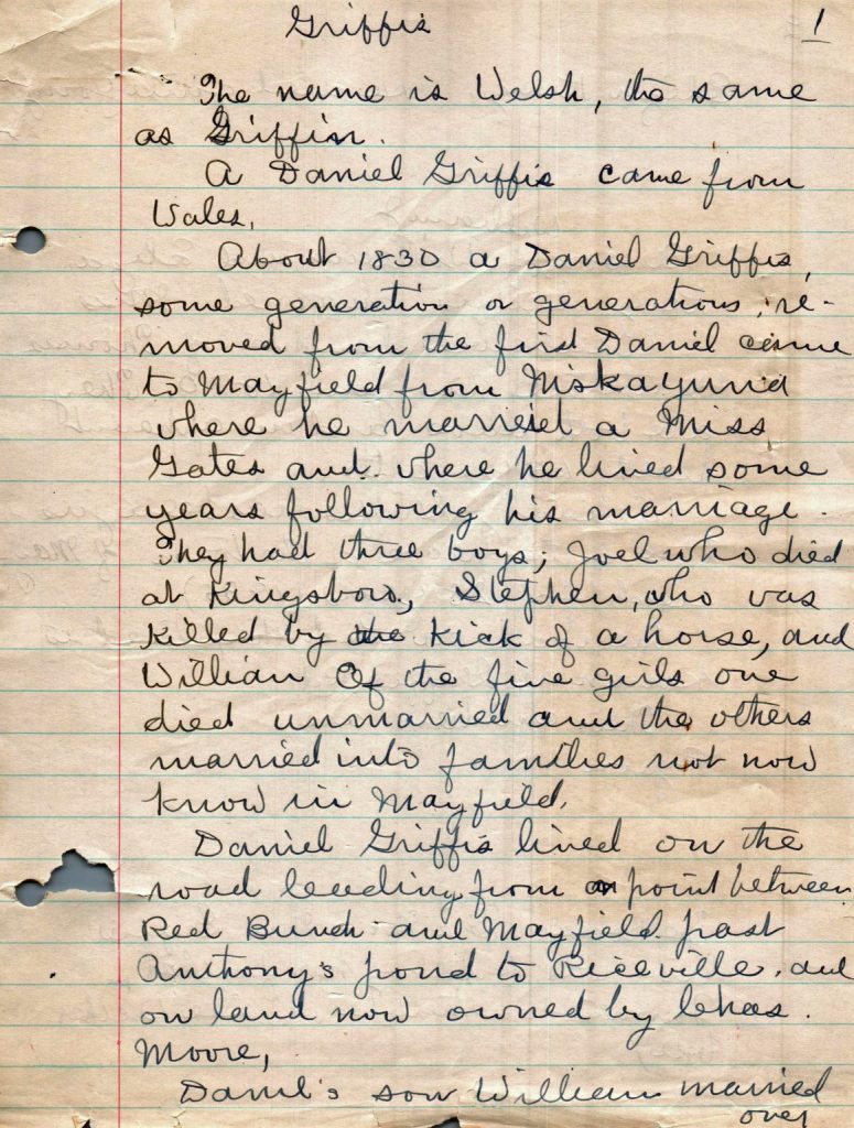
[26] Ibid
[27] See: John Rowlands, The Homes of Surnames in Wales in John Rowlands and Shiela Rowlands, ed, Stages in Researching Welsh Ancestry. Bury, England: The Federation of Family History Societies Publications Ltd., 1999. Page 162
[28] Distribution of Griffith and Griffiths Head of Households by Welsh County 1881
| County | Sur- name Griff- ith/iths | Sur- name Rank of top 300 sur- Names / County | Number of House- holds in county | Percentage of Griffith and Griffiths Households Across Counties | Percentage of Griffiths Households Across Counties |
|---|---|---|---|---|---|
| Anglesey | ith | 14th | 722 | 2.4 % | |
| iths | 0 | 0 | 0 | ||
| Brecknock | ith | 175th | 24 | 3.2% | |
| iths | 12th | 937 | 3.9% | ||
| Caernarfon | ith | 10th | 2954 | 15.7% | |
| iths | 12th | 1697 | 7.1% | ||
| Cardigan | ith | 70th | 25 | 4.6% | |
| iths | 13th | 1330 | 5.6% | ||
| Carmarthen | ith | 73rd | 78 | 10.0% | |
| iths | 8th | 2842 | 11.9% | ||
| Denbigh | ith | 30th | 275 | 6.8% | |
| iths | 10th | 1726 | 7.2% | ||
| Flinshire | ith | 64th | 106 | 5.8% | |
| iths | 9th | 1626 | 6.8% | ||
| Glamorgan | ith | 66th | 640 | 27.0% | |
| iths | 10th | 7362 | 30.7 | ||
| Merioneth | ith | 19th | 618 | 2.7% | |
| iths | 12th | 787 | 3.3% | ||
| Monmouth | ith | 0 | 0 | 5.4% | |
| iths | 19th | 1605 | 6.7% | ||
| Montgomery | ith | 84th | 76 | 4.0% | |
| iths | 14th | 1095 | 7.9 | ||
| Penbroke | ith | 84th | 110 | 10.4% | |
| iths | 6th | 2974 | 12.4 |
[29] See Griffis, Jim, Y-DNA and the Griffis Paternal Line – Part One, 26 Sep 2022, Griffis Family: Selected Stories from the Past, https://griffis.org/y-dna-and-the-griffis-paternal-line-part-one/
[30] Things that DNA tests cannot do:
Y-DNA tests can not tell you if your paternal line was from a particular culture or tribe, or some other group in the past. If based on the results of your DNA test you connect with another person in a Y-DNA project who had documentation of this knowledge, then indirectly the DNA test can provide leads to document this specific fact. One does not learn about this information through Y-DNA. Certain genetic configurations of designated markers of Y-DNA have been found in human remains in areas inhabited by specific ancient cultures. The results of various studies indicate that specific Y-DNA spread historically in general geographic areas at certain, general time periods. The mapping of ancient DNA distributions are more precise in the last ten years but as to whether one’s ancestors spent time among a particular culture is completely unknown. Current knowledge reflects that we do not know where all the Y-DNA mutations started. We have an idea of what cultures certain Y-DNA may have traveled with but that does not mean anyone’s specific ancestors traveled with them and did not travel with another culture.
DNA tests per se can not break brick walls encountered in ancestry research. DNA tests can help to break through brick wall but only with help. Typically the test results will facilitate finding other individuals with knowledge or documentation that helps you break through your own brick wall because they knew something farther back that you did, or you put your two sets of knowledge together and you find discoveries based on common ancestors.
Y-DNA tests can not identify specific ancestors or where they lived. The original, geographical locations and names of ancestors can be determined through traditional historical sources based on genetic lines that may be discovered.
Y-DNA tests can not identify the exact generation of a common ancestor with supporting data. Age estimation of a common ancestor has a large margin of error and is a topic of contention among DNA companies and scientists.
[31] The best Y-DNA tests at the time of my testing was from FamilyTreeDNA (FTDNA). They are the only company of to offer dedicated Y testing and the only company that provides matching capabilities based on other testers who may post gnealological trees with supporting information. FamilyTreeDNA offers three levels of Y-DNA STR testing: Y-37, Y-111, and Big Y-700 (Big Y also tests SNPs). The numbers refer to how many DNA markers the test examines. The more markers, the more useful the results will be. They also have the largest population of Y-DNA testers.
See: Y-DNA SNP testing chart, Y-DNA SNP testing chart, Y-DNA STR testing comparison chart, International Society of Genetic Genealogy Wiki, This page was last edited on 16 February 2022, page accessed 20 Feb 2022, https://isogg.org/wiki/Y-DNA_SNP_testing_chart
Y-DNA STR testing comparison chart, International Society of Genetic Genealogy Wiki, This page was last edited on 11 July 2022, https://isogg.org/wiki/Y-DNA_STR_testing_comparison_chart
Marc McDermott, Best Y-DNA Test: Everything you need to know about Y-DNA testing for genealogy, 17 Nov 2021, smarterhobby.com, https://www.smarterhobby.com/genealogy/best-y-dna-test/
Genealogical DNA Test, Wikipedia, This page was last edited on 11 August 2022, page accessed 12 Aug 2022,https://en.wikipedia.org/wiki/Genealogical_DNA_test
Diahan Southard, What’s the Big Y-700 Test? Should I Choose a Y-DNA Test?, Family Tree Magazine, Jan / Feb/ 2018, https://familytreemagazine.com/dna/big-y-700/
Y-chromosome DNA (Y-DNA),FamilyTreeDNA Help Center, Page accessed 14 Aug 2022, https://help.familytreedna.com/hc/en-us/articles/4414463886351-Y-chromosome-DNA-Y-DNA-#y-dna-snps-0-0
2020 Review Of Big Y, FamilyTreeDNA Blog, 1 Feb 2021, https://blog.familytreedna.com/2020-review-of-big-y/
Big Y-700 Tests: Any advice for advanced analysis of results?, WikiTree G2G, 19 Apr 2021, https://www.wikitree.com/g2g/1223388/big-y-700-tests-any-advice-for-advanced-analysis-of-results
Big Y, FamilyTreeDNA Blog, not dated, https://blog.familytreedna.com/wp-content/uploads/2021/05/big-y.pdf
2019 Review Of Big Y, FamilyTree DNA Blog, 27 Dec 2019, https://blog.familytreedna.com/2019-review-of-big-y/
Roberta Estes Y-700: The Forefront of Y Chromosome Testing, 7 Jun 2017, FamilyTree DNA Blog, https://blog.familytreedna.com/human-y-chromosome-testing-milestones/
Roberta Estes, FamilyTree DNA Blog, Why Big Y-700? 21 Oct 2022, https://blog.familytreedna.com/why-big-y-700/
[32] J. David Vance, DNA Concepts for Genealogy: Y-DNA Testing Part 1, 10 Oct 2019, https://youtu.be/RqSN1A44lYU Part 1 of a 3-part introduction series to Y-DNA for genealogists. This first video focuses on “Why?” use Y-DNA for genealogy – what benefits does it offer and why should genealogists consider using Y-DNA as part of their research?
J. David Vance, DNA Concepts for Genealogy: Y-DNA Testing Part 2, 3 Oct 2019 https://www.youtube.com/watch?v=mhBYXD7XufI&t=355s Part 2 of a 3-part introduction series to Y-DNA for genealogists. This second video focuses on “What?” for Y-DNA for genealogy – what are STRs and SNPs, what is genetic distance, what is the haplotree, and other related questions
J. David Vance, DNA Concepts for Genealogy: Y-DNA Testing Part 3, 10 Oct 2019 https://www.youtube.com/watch?v=03hRXVg9i1k&t=4sPart 3 of a 3-part introduction series to Y-DNA for genealogists. This third video focuses on “How?” for Y-DNA for genealogy – how do I use the information provided by Y-DNA tests to advance my genealogy and/or my lineages?
J David Vance, The Genealogist Guide to Genetic Testing, 2020 https://www.amazon.com/Genealogists-Guide-Testing-Genetic-Genealogy/dp/B085HQXF4Z/ref=tmm_pap_swatch_0?_encoding=UTF8&qid=&sr=
Michael Hébert, Y-DNA Testing Company STR Marker Comparison Chart, Last updated on January 08, 2012, http://www.gendna.net/ydnacomp.htm
Estes, Roberta, Y DNA: Part 1 – Overview, 2 Jan 2020, DNAeXplained, https://dna-explained.com/2020/01/02/y-dna-part-1-overview/
Roberta Estes, Working with Y DNA – Your Dad’s Story, FamilyTree DNA Blog. 5 Jun 2017, https://dna-explained.com/2017/06/05/working-with-y-dna-your-dads-story/
Roberta Estes, STRs vs SNPs, Multiple DNA Personalities, DNAeXplained – Genetic Genealogy, 10 Feb 2014, https://dna-explained.com/2014/02/10/strs-vs-snps-multiple-dna-personalities/
Y chromosome DNA tests, International Society of Genetic Genealogy Wiki, This page was last edited on 6 September 2024, https://isogg.org/wiki/Y_chromosome_DNA_tests
[33] Chris Gunter, Single Nucleotide Polymorphisms (SNPS), 10 May 2022, National Human Genome Research Institute, https://www.genome.gov/genetics-glossary/Single-Nucleotide-Polymorphisms
What are single nucleotide polymorphisms (SNPs)?, MedlinePlus, National Library of Medicine, https://medlineplus.gov/genetics/understanding/genomicresearch/snp/
Single-nucleotide polymorphism, Wikipedia, page was last edited on 11 November 2022, https://en.wikipedia.org/wiki/Single-nucleotide_polymorphism
SNP’s, Genetics Generation, https://knowgenetics.org/snps/
Making SNPs Make sense, Learn Genetics, Genetic Science Learning Center, https://learn.genetics.utah.edu/content/precision/snips
[34] STRs vs SNPs, Multiple DNA Personalities, DNAeXplained – Genetic Genealogy, 10 Feb 2014, https://dna-explained.com/2014/02/10/strs-vs-snps-multiple-dna-personalities/
STR Analysis, Wikipedia, page was last edited 25 Oct 2022, https://en.wikipedia.org/wiki/STR_analysis
Microsatellite, Wikipedia, page was last edited 25 Oct 2022, https://en.wikipedia.org/wiki/Microsatellite
Terry Taylor, What is STR Analysis?, 2 Mar 2011, This article appeared in NIJ Journal Issue 267, March 2011, as a sidebar to the article Extending the Time to Collect DNA in Sexual Assault Cases by Terry Taylor.
Has Fan, Jai-You Chu, A Brief Review of Short Tandem Repeat Mutation, Genomics Proteomics Bioinformatics. 2007; 5(1): 7–14. Published online 2007 Jun 15. doi: 10.1016/S1672-0229(07)60009-6
Short Tandem Repeat, International Society of Genetic Genealology Wiki, page was last edited on 31 January 2017, https://isogg.org/wiki/Short_tandem_repeat
Michael Hébert, Y-DNA Testing Company STR Marker Comparison Chart, Last updated on January 08, 2012, http://www.gendna.net/ydnacomp.htm
Kayser et al. (2004), A Comprehensive Survey of Human Y-Chromosomal Microsatellites Am. J. Hum. Genet., 74 1183-1197. NB online only data file
Krahn, Thomas. “Y-STR fingerprint – Panels” (PDF). Price List DNA-Fingerprint – Genealogy Testing Services. Retrieved 11 August 2012.
Butler, John M. (9 January 2012). “Y-Chromosome STRs”. Short Tandem Repeat DNA. NIST Standard Reference Database SRD 130. Retrieved 11 August 2012.
Butler, John; Kline, Decker (2009-06-29). “Summary List of Y Chromosome STR Loci and Available Fact Sheets”. NIST Standard Reference Database SRD 130. Retrieved 11 August 2012.
State of the Y-Chromosome for Human Identity Testing: John Butler talk at Canadian Forensic DNA Technology Workshop (June 8, 2005)
Y STR Positions along Y Chromosome, STRBase (SRD-130) National Institute of Standards and technology,, U.S. Department of Commerce, https://strbase.nist.gov//ystrpos1.htm
Y-STR Reference Bibliography, STRBase (SRD-130) National Institute of Standards and technology, U.S. Department of Commerce, https://strbase.nist.gov//ystr_ref.htm
SNP-based age analysis methodology: a summary, Summarised description of the age analysis pipeline — Iain McDonald, June 2017, https://www.jb.man.ac.uk/~mcdonald//genetics/pipeline-summary.pdf
Albers PK, McVean G (2020) Dating genomic variants and shared ancestry in population-scale sequencing data. PLoS Biol 18(1): e3000586. https://doi.org/10.1371/journal.pbio.3000586
National Library of Medicine, Genetics, What are single nucleotide polymorphisms (SNPs)? Page accessed 1 Oct 2022, https://medlineplus.gov/genetics/understanding/genomicresearch/snp/
[35] Jim Griffis, Y-DNA and the Griffis Paternal Line Part Three: The One-Two Punch of Using SNPs and STRs, February 23, 2023, Griffis Family: Selected Stories from the Past, https://griffis.org/y-dna-and-the-griffis-paternal-line-part-three-the-one-two-punch-of-using-snps-and-strs/
[36] Rob Spencer, STR Clades, Tracking Back: a website for genetic genealogy tools, experimentation, and discussion, http://scaledinnovation.com/gg/gg.html?rr=strclades
[37 Rob Spencer, The Big Picture of Y STR Patterns, The 14th International Conference on Genetic Genealogy, Houston, TX March 22-24, 2019, http://scaledinnovation.com/gg/ext/RWS-Houston-2019-WideAngleView.pdf Page 11
[38] Y-SNP & Y-STR Tools Used in Y-DNA Research:
| STR / SNP Tool | Creator | Description |
|---|---|---|
| SNP Tracker | Spencer | Creates a map based on SNP data which traces paternal line from human origins |
| Britain & Ireland SNP & Surname Mapper | Spencer | Based on Surname or SNP input, provides historic British census countywide data and maps |
| Y STR Clustering and Dendrogram Drawing | Spencer | Generate circular/ linear dendrograms from FTDNA data. The tool provides quick and incisive graphic depictions of relationships between test kits on STR values and genetic distance. |
| FTDNA Admin Utilities | Spencer | SNP Breadcrumbs; Find Common Ancestor; Export Tree Text; ISOGG Y-SNP Synonyms; |
| Still Another Phylogeny Program SAPP | Vance | Import Y-STR and Y-SNP data to create phylogenetic tree. This is a great program to use in conjunction with SNP results that group test results in a major SNP rant. The tool can then map out possible lines between testers based on STR values. |
| Y-DNA Matches | FTDNA | Lists Matches based on Y 12, 25, 37, 67, 111, and Big Y 700 STR tests |
| Y-DNA Haplotree | FTDNA | Lists haplotree based on confirmed terminal haplogroup, lists all SNPs tested positive or presumed positive |
| Y-STR Results | FTDNA | Lists the specific test results for Y-111 and Big Y 700 STR tests |
| Big Y BlockTM Tree | FTDNA | A vertical-block visual diagram of Y-DNA haplotree showing Big Y testers. This tool helps you visualize how the paternal lineages are related to each other. Also provides Paternal Countries of Origin and other information. |
| Haplogroup Story | FTDNA | Part of FamilyTreeDNA Discover™ series reports. Based on SNP input, provides estimated time of when haplogroup was born. when did your paternal ancestor live and where are his descendants found today. |
| FTDNATiP™ Report | FTDNA | Provides Genetic Distance estimates for potential Y-DNA STR matches |
[39] The term “haplotype” refers to the inheritance of a cluster of single nucleotide polymorphisms (SNPs), which are variations at single positions in the DNA sequence among individuals.
A modal haplotype is the most commonly occurring haplotype (a set of STR marker values) derived from the DNA test results of a specific group of people. The modal haplotype does not necessarily correspond with the ancestral haplotype – the haplotype of the most recent common ancestor.
Biesecker, Leslie, Haplotype, National Institute of Human Genome Research Institute, https://www.genome.gov/genetics-glossary/haplotype
Haplotype, Wikipedia, This page was last edited on 19 September 2024, https://en.wikipedia.org/wiki/Haplotype
Genotyping: Terms to know, Integrated DNA Technologies, https://www.idtdna.com/pages/education/decoded/article/genotyping-terms-to-know
Haplotypes: a cut-out-and-keep guide, 12 Mar 2021, Genomics Education Programme, https://www.genomicseducation.hee.nhs.uk/blog/haplotypes-a-cut-out-and-keep-guide/
A haplotree is a branching diagram that shows evolutionary relationships between biological species based on their genetic characteristics. It represents the genetic journey of human populations and illustrates how different groups are related through common ancestors. Each branch represents thousands or tens of thousands of years of genetic changes, helping identify deep ancestral origins.
The Y-DNA haplotree is a phylogenetic tree that represents the evolutionary relationships and genetic diversity of human Y chromosomes. It is a branching diagram that looks like a family tree that shows the inferred evolutionary connections among different Y-DNA haplogroups, which are defined by specific mutations in the SNP portions of the male-specific Y chromosome.
Haplogroups are named using a system developed by the Y Chromosome Consortium (YCC), which uses a combination of letters, numbers, and SNP (Single Nucleotide Polymorphism) markers.
FamilyTreeDNA, in collaboration with the National Geographic Genographic Project, has created one of the largest and most comprehensive Y-DNA haplotrees. This tree is continuously updated as new SNPs are discovered through advanced testing methods like Big Y DNA test, allowing for increasingly detailed branching and more precise placement of individuals within the tree.
See:
Human Y-chromosome DNA haplogroup, Wikipedia, This page was last edited on 5 October 2024, https://en.wikipedia.org/wiki/Human_Y-chromosome_DNA_haplogroup
Y chromosome DNA haplogroup, International Society of Genetic Genealogy, This page was last edited on 1 July 2021, https://isogg.org/wiki/Y_chromosome_DNA_haplogroup
Y-DNA Haplogroup Tree 2019-2020, International Society of Genetic Genealogy, Version: 15.73 Date: 11 July 2020, https://isogg.org/tree/
Estes, Roberta, Family Tree DNA’s PUBLIC Y DNA Haplotree, 27 Sep 2018, DNAeXplained, https://dna-explained.com/2018/09/27/family-tree-dnas-public-y-dna-haplotree/
[40] For a list of all the equivalent SNPs in the Griff(is)(es)(ith) line, see Jim Griffis, Y-DNA and the Griffis Paternal Line Part Three: The One-Two Punch of Using SNPs and STRs, February 23, 2023, Footnote [18] , https://griffis.org/y-dna-and-the-griffis-paternal-line-part-three-the-one-two-punch-of-using-snps-and-strs/
[41] The decline of G2a’s dominance occurred through multiple replacements. Local hunter-gatherers carrying the I2 haplogroup genetic line first replaced many G2a lineages, likely through violent takeover of agricultural societies. The most significant replacement came with Indo-European expansions, primarily through the R1a haplogroup becoming prevalent in Eastern Europe and parts of Scandinavia; and the R1b haplogroup becoming dominant in Western Europe.
Hay, Maciamo, Haplogroup G2a (Y-DNA) Jul 2023, Eupedia, https://www.eupedia.com/europe/Haplogroup_G2a_Y-DNA.shtml
Genetic history of Europe, Wilkpedia, This page was last edited on 8 December 2024, https://en.wikipedia.org/wiki/Genetic_history_of_Europe
A 2022 study on the effect of Y chromosome variation on coronary artery disease and mortality in the United Kingdom documented the fact that the G Haplogroup is a minority Y-Haplogroup in Great Britain. The study gathered data on males from 90 haplogroups to conduct the study.
The following Map reflects the density of representation of the G P15 haplogroup, of which the Griffis family paternal line descends from. It documents the presence of the G haplogroup in the southern region of Wales.
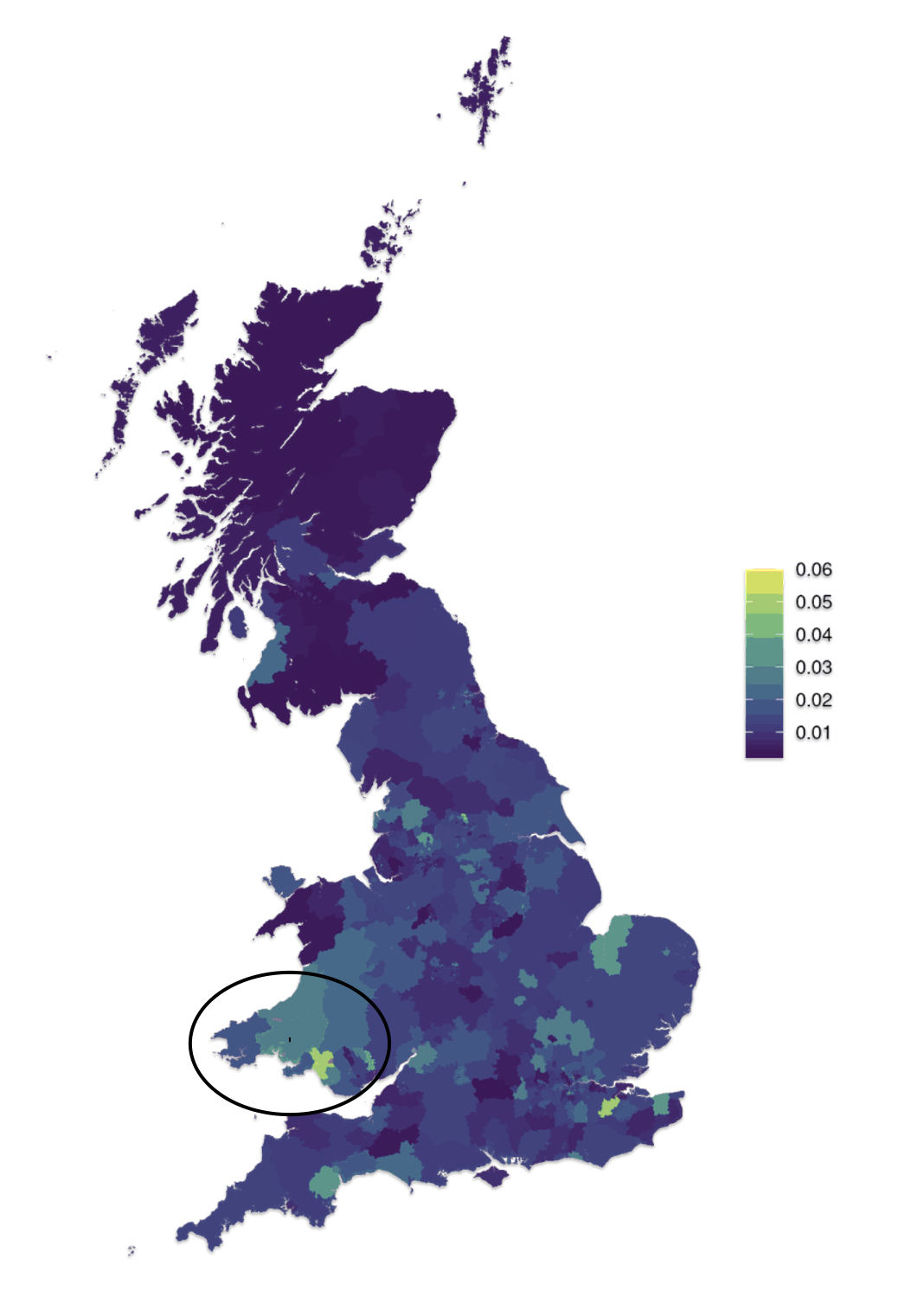
Timmers, Paul R.H.L and James F Wilson, Limited Effect of Y Chromosome Variation on Coronary Artery Disease and Mortality in the UK Biobank – Brief Report,Arteriosclerosis,Thrombosis, and Vascular Biology, Vol 42, No 9, https://doi.org/10.1161/ATVBAHA.122.317664
[42] The G2a population was severely reduced during the Indo-European expansions, particularly in northern Europe. The decimation was so thorough that modern Neolithic G2a clades or sub-branches now represent only a tiny fraction of G2a lineages in northern Europe.
Hay, Maciamo, Haplogroup G2a (Y-DNA) Jul 2023, Eupedia, https://www.eupedia.com/europe/Haplogroup_G2a_Y-DNA.shtml
Genetic history of Europe, Wilkpedia, This page was last edited on 8 December 2024, https://en.wikipedia.org/wiki/Genetic_history_of_Europe
[43] Estes, Roberta, Glossary – Terminal SNP, 29 Nov 2017, DNAeXplained, https://dna-explained.com/2017/11/29/glossary-terminal-snp/
Y-DNA project help, International Society of Genetic Genealogy Wiki, This page was last edited on 28 October 2022, https://isogg.org/wiki/Y-DNA_project_help
Let’s All Start Using Terminal SNP Labels Instead of Y Haplogroup Subclade Names, Okay?, 20 Sep 2012, Your Genetic Genealogist, http://www.yourgeneticgenealogist.com/2012/09/lets-all-start-using-terminal-snp.html
[44] Terminal SNPs can have different names across platforms because the lab or entity that discovers a SNP gets naming rights, leading to multiple naming conventions. This has resulted in a situation where the same SNP mutation can have several different names.
Each testing company or research organization uses their own prefix when naming newly discovered SNPs. For example:
- FTDNA uses their own naming convention
- YFull names SNPs from their interpretation of BAM files
- Other labs and organizations use their own prefixes.
Sometimes a single SNP mutation is discovered and named by multiple entities around the same time, resulting in dual naming. While some organizations list all equivalent SNP names, FTDNA typically selects just one name to represent the branch on their tree.
Estes, Roberta, Haplogroups, SNPs and Family Group Confusion, 23 Jun 2014, DNAeXplained-Genetic Genealogy, https://dna-explained.com/2014/06/23/haplogroups-snps-and-family-group-confusion/
Estes, Roberta, New Y DNA Haplogroup Naming Convention, 31 Mar 2013, DNAeXplained – Genetic Genealogy, https://dna-explained.com/2013/03/31/new-y-dna-haplogroup-naming-convention/
YFull Tutorial, https://www.yfull.com/tutorial/
[45] The Chart was developed by the FamilyTreeDNA based G-L497 working group. The project includes men with the L497 SNP mutation or reliably predicted to be G-L497+ on the basis of certain STR marker values. The primary goal of the project is to identify new subgroups of haplogroup G-L497 which will provide better focus to the migration history of haplogroup G-L497 ancestors.
[46] Globetrekker is a mapping feature from FamilyTreeDNA for Big Y DNA test customers that traces paternal ancestral migration paths from Y-Adam in Africa (approximately 200,000 years ago) to recent times. The tool combines genetic data with geographical and historical information to map likely migration routes. The system continues to expand, with over 1,000 new migration paths added since its launch in July 2023, bringing the total to more than 49,000 unique paths.
Estes, Roberta, Globetrekker – A New Feature for Big Y Customers From FamilyTreeDNA, 4 Aug 2023, DNAeXplained – Genetic Genealogy, https://dna-explained.com/2023/08/04/globetrekker-a-new-feature-for-big-y-customers-from-familytreedna/
Runfeldt, Goran, Globetrekker, Part 1: A New FamilyTreeDNA Discover™ Report That Puts Big Y on the Map, 31 Jul 2023, FamilyTreeDNA Blog, https://blog.familytreedna.com/globetrekker-discover-report/
Globetrekker, Part 2: Advancing the Science of Phylogeography, 15 Aug, 2013, FamilyTreeDNA Blog, https://blog.familytreedna.com/globetrekker-analysis/
Vilar, Miguel, Globetrekker, Part 3: We Are Making History, 26 Sep 2023, FamilyTreeDNA Blog, https://blog.familytreedna.com/globetrekker-history/
[47] Haplogroup G-P303, Wikipedia, This page was last edited on 30 August 2022, https://en.wikipedia.org/wiki/Haplogroup_G-P303
[48] Ibid
[49] A dendrogram is a tree-like diagram that visualizes hierarchical relationships between objects or data points. It consists of branches (called clades) that stack and break down into smaller branches, with individual elements at the lowest level.
[50] Spencer, Rob, Y STR Clustering and Dendrogram Drawing, Dec 2024, https://scaledinnovation.com/gg/clustering.html
[51] First sentence of Chapter One, Board for Certification of Genealogists, Genealogy Standards Nashville: Turner Publishing Co., 2021
[52] Elizabeth Shown Mills, Working with Historical Evidence: Genealogical Principles and Standards, Vol 87, No. 3, Sep 1999, Evidence, A special Issue of the National Genealogical Society Quarterly, Pages 169, https://www.historicpathways.com/download/workwthhistevidence.pdf.
[53] The social sciences do have research standards, especially regarding research ethics and understanding the advantages and limitations of using various approaches to gathering information and interpreting research results. These standards are more decentralized across different disciplines and professional bodies compared to the standards in genealogy. Social science standards also tend to be more provisional and debated as the fields grapple with issues of reliability and transparency.
Major social science disciplines have professional associations that establish ethical guidelines and best practices for research and teaching. For example:
- The American Psychological Association (APA) has an Ethics Code that sets standards for psychologists.
- The American Sociological Association (ASA) has a Code of Ethics outlining professional responsibilities for sociologists.
- The American Anthropological Association (AAA) has a Code of Ethics and Principles of Professional Responsibility.
These ethics codes cover issues like protecting research participants, avoiding discrimination, maintaining confidentiality, and representing findings accurately. They aim to uphold the integrity of the disciplines.
If we look at the social sciences as professional organizations, what is firmly grounded in the social sciences is the provision of research training: how to conduct research and how to document research. Universities and colleges become their ‘gatekeepers’ for training prospective members of their organization. Each social science discipline has basic formal core courses in undergraduate and graduate studies in qualitative and quantitative research methods, theory, statistics, and other areas pertinent to each social science discipline.
Social scientists are expected to use rigorous, systematic methods in their data collection, research, and analysis. Quantitative research should follow established statistical practices. Qualitative research should be conducted according to methodological standards for interviews, ethnography and content analysis. There are also general goals for transparency in social science research: making data, materials, and analysis code publicly available to allow others to scrutinize and reproduce findings.
As in other academic fields, social scientists submit their research to peer-reviewed journals, where other experts evaluate the work before publication. Peer review is seen as essential for maintaining standards. Many social scientists also believe findings need to be replicated by other researchers before being considered conclusive. Replication helps guard against false positives and ensures results are reliable. Historically, replication attempts have been relatively rare compared to original studies.
Social scientists use various methods to ensure the accuracy and reliability of their research findings. Social scientists carefully design their studies to minimize potential sources of bias or error. Each social science discipline has established methodological standards and best practices that researchers are expected to follow. This involves:
- Well-designed studies to provide a strong foundation for accurate results.;
- Clearly defining the research question and hypotheses;
- Selecting appropriate sampling methods to ensure the sample is representative of the population of interest;
- Choosing reliable and valid measurement instruments;
- Using control groups and randomization in experiments to isolate causal effects; and
- Collecting data systematically and consistently.
American Sociological Association, Code of Ethics and Policies and Procedures of the ASA Committee on Professional Ethics, Washington: American Sociological Association, 208,
https://www.asanet.org/wp-content/uploads/savvy/images/asa/docs/pdf/CodeofEthics.pdf
Quick Style Guide, Washington: American Sociological Association 2007, http://www.asanet.org/students/Quick%20Style%20guide.pdf
American Educational Research Association, Standards for Reporting on Empirical Social Science Research in AERA Publications, Educational Researcher, Vol. 35, No. 6, August / September, 2006, pp. 33–40, https://www.aera.net/Portals/38/docs/12ERv35n6_Standard4Report%20.pdf
American Anthropological Association Policies, https://americananthro.org/about/policies/
APA-approved standards and guidelines, American Psychological Association, https://www.apa.org/research-practice/standards-guidelines
American Economic Association, Best Practices for Economists, https://www.aeaweb.org/resources/best-practices
[54] Historical analysis and methods refer to the techniques and guidelines historians use to research and interpret the past. For historians, the goal is to construct an accurate and reliable account of past events by critically examining and synthesizing evidence from primary and secondary sources.
History is fundamentally about making arguments and interpretations based on the available evidence. Historians situate their arguments within existing scholarship, linking their new interpretations to previous work while noting how new evidence may require revising past narratives.
Well-supported historical arguments consider counter-evidence, multiple causation, and avoid unsupported speculation. Historians explicitly distinguish between opinion and hypotheses grounded in evidence. Historical analysis and methods are the tools historians use to rigorously examine the past and construct meaningful, evidence-based interpretations. It is a complex process requiring research skills, critical analysis, and argumentation to produce works that deepen our understanding of history.
With the risk of over simplification, historians rely on two main types of sources:
- Primary sources are direct evidence from the time period being studied, such as letters, diaries, artifacts, or eyewitness accounts.
- Secondary sources are created later by someone who did not experience the events firsthand, such as scholarly books and articles.
Historians must carefully assess the credibility and biases of each source. After collecting evidence, historians analyze the facts to construct a coherent narrative about the past. This involves:
- Looking for patterns, cause-and-effect relationships, and the influence of individuals, ideas, and chance events;
- Considering multiple perspectives and motivations of historical figures;
- Comparing and contrasting differing sets of ideas and institutions; and
- Drawing comparisons across time periods and regions to identify long-term developments.
Historians use critical textual analysis as a key method in evaluating historical sources and constructing reliable interpretations of the past. This involves carefully examining the content, context, and origins of texts to assess their credibility and meaning. Historians consider who created a source and their potential biases or motivations that could influence the content. Key questions include:
- What was the author’s background, position, and possible agenda?
- Did they have firsthand knowledge of the events described or a particular perspective?
- How might the intended audience have shaped what was written?
Recognizing the “tendency” or bias of a source helps determine its reliability and limitations.
Well-supported historical arguments consider counter-evidence, multiple causation, and avoid unsupported speculation. Historians explicitly distinguish between opinion and hypotheses grounded in evidence.
Historians cross-check sources against each other to assess consistency and reliability. The more independent sources that agree on a fact or event, the more confidence historians can have in that information. However, even a majority of sources agreeing does not guarantee accuracy without passing the test of critical analysis. Historians also consider how the values and ideas of the time period and cultural context may have influenced a source’s content.
See for example:
Gunn, Simon and Lucy Faire, eds, Research Methods for History, Edinburg: Edinburgh University Press, 2012
Schrag, Zachary, The Princeton guide to historical research, Princeton: Princeton University Press, 2021
Shafer, Robert Jones, A guide to historical method, Homewood, Ill. : Dorsey Press, 1974
Brundage, Anthony, Going to the sources : a guide to historical research and writing, Hoboken, New Jersey : John Wiley & Sons Inc., 2017
Hudson, Pat, History by numbers : an introduction to quantitative approaches, London : Arnold ; New York : Co-published in the U.S.A. by Oxford University Press, 2000
Todd,Molly, Undergraduate research in history : a guide for students, Abingdon, Oxon ; New York, NY : Routledge, 2022
Dobson, Miriam and Benjamin Ziemann , ed,Reading primary sources : the interpretation of texts from nineteenth and twentieth century history, London ; New York, New York : Routledge, 2020
[55] See for example:
Elizabeth Shown Mills, Bridging the Historic Divide: Family History and “Academic” History, “History or Genealogy? Why Not Both?” presented at the Indianapolis-based Midwestern Roots Conference, Sponsored jointly by the Indiana Historical Society and the Indiana Genealogy Society, August 2004, https://www.historicpathways.com/download/bridghisdivideivide.pdf
Elizabeth Shown Mills, Academia vs. Genealogy Prospects for Reconciliation, National Genealogical Society Quartrerly, Volume 71 , Number 2, June 1983, Pages 99 – 106 ,https://www.historicpathways.com/download/acadvgenea.pdf
Elizabeth Shown Mills, Genealogy in the “Information Age”: History’s New Frontier?, national Genealogical Society Quarterly 91 (December) 2003, Pages 260-277, https://historicpathways.com/download/genininfoage.pdf
Taylor, Robert & Ralph J. Crandall, Historians and Genealogists: An Emerging Community of Interest, Chapter One in Robert M. Taylor & Ralph J. Crandall, Eds., General and Change: Genealogical Perspectives in Social History, Macon: Mercer University Press, 1986, Pages 3 – 28
Hays, Samuel P., History and Genealogy: Patterns of Change and Prospects for Cooperation, Cahpeter Two in Robert M. Taylor & Ralph J. Crandall, Eds., General and Change: Genealogical Perspectives in Social History, Macon: Mercer University Press, 1986, Pages 29 –
[56] ICAPGen focuses more on demonstrating deep expertise in a specific geographical area, while BCG credentials validate a genealogist’s ability to apply professional research standards across any region. But both credentials mark one as a ‘qualified professional’ genealogist who effecetively can serve clients.
- ICAPGen awards the Accredited Genealogist (AG®) credential. BCG offers two credentials: Certified Genealogist (CG℠) and Certified Genealogical Lecturer (CGL℠).
- ICAPGen requires applicants to specialize in one of over 25 geographical regions (e.g. Germany, New York, Ireland). BCG does not require regional specialization for the CG credential.
- ICAPGen has a multi-step process including a readiness assessment, four-generation project, two timed tests, and an oral review. BCG requires submission of a single portfolio of work samples demonstrating various research skills.
- The BCG portfolio includes a code of ethics, development activities, document work, research report, case study, and kinship-determination project. ICAPGen does not have a single portfolio, but incorporates some similar elements across its multi-step process.
- BCG places a strong emphasis on adherence to the Genealogical Proof Standard throughout the portfolio. ICAPGen incorporates professional standards like the GPS, but the focus is more on regional expertise.
- Those with a CG or AG in one region can apply for the other credential with reduced experience requirements.
See:
Why Become an AG Professional, The International Commission for the Accreditation of Professional Genealogists, https://www.icapgen.org/become-accredited/
Accredited genealogists and certified genealogists: Different credentials that both lead to quality research, Heritage Bridge, https://www.heritagebridge.com/blog/2022/3/9/accredited-genealogists-and-certified-genealogists-different-credentials-that-both-lead-to-quality-research
Credentialing: Accreditation, Certification, or Both?, May 30, 2013, Board for Certification of Genealogists, https://bcgcertification.org/credentialing-accreditation-certification-or-both/
Genealogy Degrees and Accreditations, Legacy Tree Genealogists, https://www.legacytree.com/blog/genealogy-degrees-and-accreditations
[57] Hjorthén Adam , Reframing the History of American Genealogy: On the Paradigm of Democratization and the Capitalization of Longing. Genealogy. 2022; 6(1):21. https://doi.org/10.3390/genealogy6010021
Elizabeth Shown Mills, Working with Historical Evidence: Genealogical Principles and Standards, Vol 87, No. 3, Sep 1999, Evidence, A special Issue of the National Genealogical Society Quarterly, Page 169, https://www.historicpathways.com/download/workwthhistevidence.pdf.
Elizabeth Shown Mills, Genealogy in the “Information Age”: History’s New Frontier?, national Genealogical Society Quarterly 91 (December) 2003, Pages 260-277, https://historicpathways.com/download/genininfoage.pdf
[58] Elizabeth Shown Mills, Working with Historical Evidence: Genealogical Principles and Standards, Vol 87, No. 3, Sep 1999, Evidence, A special Issue of the National Genealogical Society Quarterly, Page 167-169, https://www.historicpathways.com/download/workwthhistevidence.pdf.
[59] Elizabeth Shown Mills, Working with Historical Evidence: Genealogical Principles and Standards, Vol 87, No. 3, Sep 1999, Evidence, A special Issue of the National Genealogical Society Quarterly, Page 169, https://www.historicpathways.com/download/workwthhistevidence.pdf.
[60] The American Genealogist (TAG), founded in 1922 by Donald Lines Jacobus, is a quarterly journal focused on carefully documented genealogical analyses and has been America’s premier independent genealogical journal.
“The American Genealogist was begun in 1922 by Donald Lines Jacobus (1887–1970) as the New Haven Genealogical Magazine. The first eight volumes consisted primarily of the editor’s alphabetical compendium of “Families of Ancient New Haven.” When that project was completed, the journal became, with the July 1932 issue, The American Genealogist and New Haven Genealogical Magazine. It was dedicated to the elevation of genealogical scholarship through carefully documented analyses of genealogical problems and through short compiled genealogies. In 1937 the subtitle was dropped, and the journal became simply The American Genealogist, usually abbreviated as TAG.”
The American Genealogist, https://americangenealogist.com
The National Genealogical Society Quarterly (NGSQ), established in 1912, publishes scholarly material covering all US regions and ethnic groups.
“Since 1912, the National Genealogical Society Quarterly has published material concerning all regions of the nation and all ethnic groups including case studies, essays on new methodology and little-known resources, critical reviews of current books, and previously unpublished source materials.“
National Genealogical Society Quarterly (NGSQ) & Archive, https://www.ngsgenealogy.org/ngsq/
The New England Historical and Genealogical Register, launched in 1847, set the standard for American genealogical writing and continues to publish historical and genealogical materials. American Ancestors set the standard for American genealogical writing in 1847 with the first issue of its quarterly journal, The New England Historical and Genealogical Register.
American Ancestor, A National Center for Family, History, Heritage and Culture, https://www.americanancestors.org/publications
The Genealogist, founded in 1980 by Dr. Neil D. Thompson, publishes high-quality genealogical articles and is now owned by The American Society of Genealogists
Hansen, Charles and Gale Ion Harris, eds, The Genealogist, American Society of Genealogists, https://fasg.org/the-genealogist/
[61] Board for Certification of Genealogists, The BCG Genealogical Standards Manual, Millennium Edition, Provo, Utah: Ancestry Publishing, 2000
Board for Certification of Genealogists, Genealogy Standards, New York: Ancestry Publishing, 2014
Koch, Andrew, 7 Steps for Fact-Checking Online Family Trees, FamilyTree, https://familytreemagazine.com/strategies/fact-check-family-trees/
Cooke, Lisa, How to Use Online Genealogy Trees and Hints Wisely, 21 Jul 2018, Lisa Cooke Blog, https://lisalouisecooke.com/2018/07/21/family-trees-reliable/
The following books are recommended for more information on genealogical research methods and the Genealogical Proof Standard:
- Greenwood, Val., The Researcher’s Guide to American Genealogy, Third Edition (Baltimore, Maryland: Genealogical Publishing Company, 2000).
- Mills, Elizabeth Shown, Evidence! Citation and Analysis for the Family Historian (Baltimore, Maryland: Genealogical Publishing Company, 1997).
- Mills, Elizabeth Shown,Evidence Explained: Citing History Sources from Artifacts to Cyberspace, 2nd Edition (Baltimore, Maryland: Genealogical Publishing Company, 2009).
- Mills, Elizabeth Shown, editor, Professional Genealogy: A Manual for Researchers, Writers, Editors, Lecturers, and Librarians (Baltimore, Maryland: Genealogical Publishing Company, 2001).
- Mills, Elizabeth Shown, QuickSheet: The Historical Biographer’s Guide to Cluster Research (the FAN Principle) (Baltimore, Maryland: Genealogical Publishing Company, 2012).
- Mills, Elizabeth Shown, QuickSheet: The Historical Biographer’s Guide to Individual Problem Analysis (Baltimore, Maryland: Genealogical Publishing Company, 2012).
- Mills, Elizabeth Shown,QuickSheet: The Historical Biographer’s Guide to the Research Process (Baltimore, Maryland: Genealogical Publishing Company, 2012).
- Rose, Christine, Genealogical Proof Standard: Building a Solid Case, 3rd Edition Revised (San Jose, California: CR Publications, 2009).
[62] Genealogical Standards and Guidelines – International Institute, FamilySearch Wiki, FamilySearch, This page was last edited on 27 April 2023, https://www.familysearch.org/en/wiki/Genealogical_Standards_and_Guidelines_-_International_Institute
Ethics and Standards, Board for Certification of Genealogists (BCG), https://bcgcertification.org/ethics-standards/
Genealogy Research Guide, Smithsoian Libraries, Last Updated October 6, 2023, https://library.si.edu/research/genealogy
National Genealogical Society, NGS Guidelines, https://www.ngsgenealogy.org/free-resources/guidelines/
Genealogical Standards and Guidelines – International Institute, FamilySearch Wiki, FamilySearch, This page was last edited on 27 April 2023, https://www.familysearch.org/en/wiki/Genealogical_Standards_and_Guidelines_-_International_Institute
Ethics and Standards, Board for Certification of Genealogists (BCG), https://bcgcertification.org/ethics-standards/
Genealogy Research Guide, Smithsoian Libraries, Last Updated October 6, 2023, https://library.si.edu/research/genealogy
National Genealogical Society, NGS Guidelines, https://www.ngsgenealogy.org/free-resources/guidelines/
[63] Lucy, Catherine, Research Trends & Emerging Technologies for Genealogists, School of Information Student Research Journal, Volume 5, Issue 2, Article 4, Jan 2015, Page 1, https://scholarworks.sjsu.edu/cgi/viewcontent.cgi?article=1217&context=ischoolsrj
[64] Kratz, Jessie, Census Records: The 72-Year Rule, 20 Jan 2022, Pieces of History, National Archives Blog, https://prologue.blogs.archives.gov/2022/01/20/census-records-the-72-year-rule/
O’Daniel, Patrick, The Primary Source: Issues in the Usability of Genealogical Records, Master of Science Thesis, Dec 2007, https://trace.tennessee.edu/cgi/viewcontent.cgi?article=1213&context=utk_gradthes
[65] Lucy, Catherine, Research Trends & Emerging Technologies for Genealogists, School of Information Student Research Journal, Volume 5, Issue 2, Article 4, Jan 2015, Page 1, https://scholarworks.sjsu.edu/cgi/viewcontent.cgi?article=1217&context=ischoolsrj
Learning and Overcoming the Challenges of Genealogical Research, 18 Jul 2018, Historical Society of Pennsylvania, https://hsp.org/blogs/fondly-pennsylvania/learning-and-overcoming-challenges-genealogical-research
[66] Ruggles S, Fitch C, Roberts E. Historical Census Record Linkage. Annu Rev Sociol. 2018 Jul;44:19-37. doi: 10.1146/annurev-soc-073117-041447. Epub 2018 May 18. PMID: 30369709; PMCID: PMC6200350. https://pmc.ncbi.nlm.nih.gov/articles/PMC6200350/
[67] Kratz, Jessie, Researching the Family Tree, Pieces of History, 25 Oct 2016, National Archives Blog, https://prologue.blogs.archives.gov/2016/10/25/researching-the-family-tree/
O’Hare, Sheila, Genealogy and History, Apr 2002, Common Place, https://commonplace.online/article/genealogy-and-history/
[68] Dyer, Nicole Elder, Genealogy Research in the 21st Century Part I: Genealogy Research is Still Hard, 20 Mar 2020, Family Locket, https://familylocket.com/genealogy-research-is-still-hard/
Mulcahy, Bryan L. How to Evaluate Genealogical Evidence , Illinois Sons of the American Revolution, https://www.illinois-sar.org/uploads/9/7/6/5/97654736/how_to_evaluate_genealogical_evidence.pdf
[69] Lucy, Catherine, Research Trends & Emerging Technologies for Genealogists, School of Information Student Research Journal, Volume 5, Issue 2, Article 4, Jan 2015, Page 2, https://scholarworks.sjsu.edu/cgi/viewcontent.cgi?article=1217&context=ischoolsrj
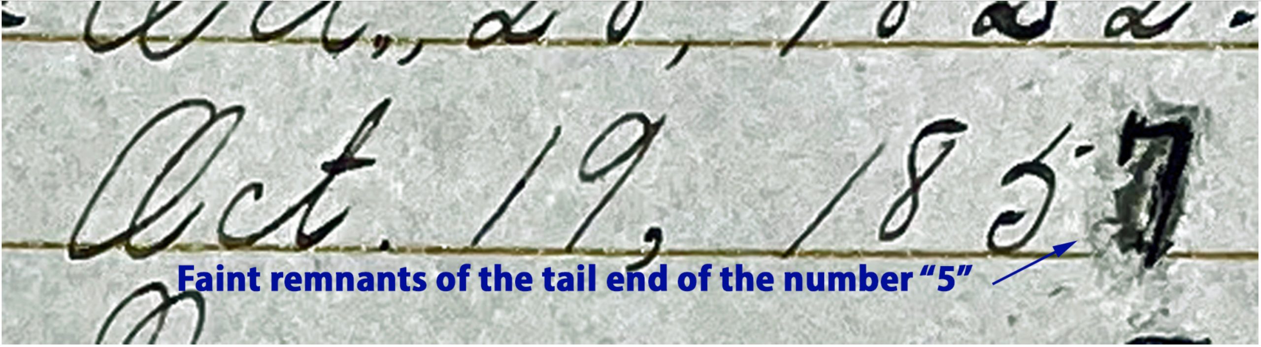
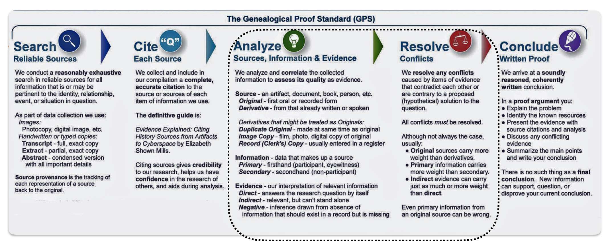
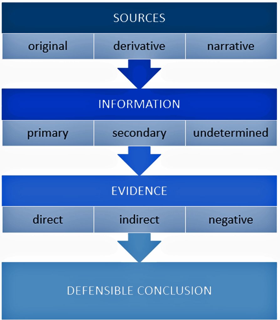
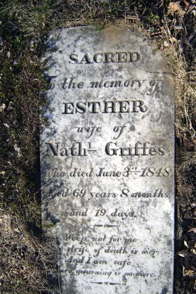
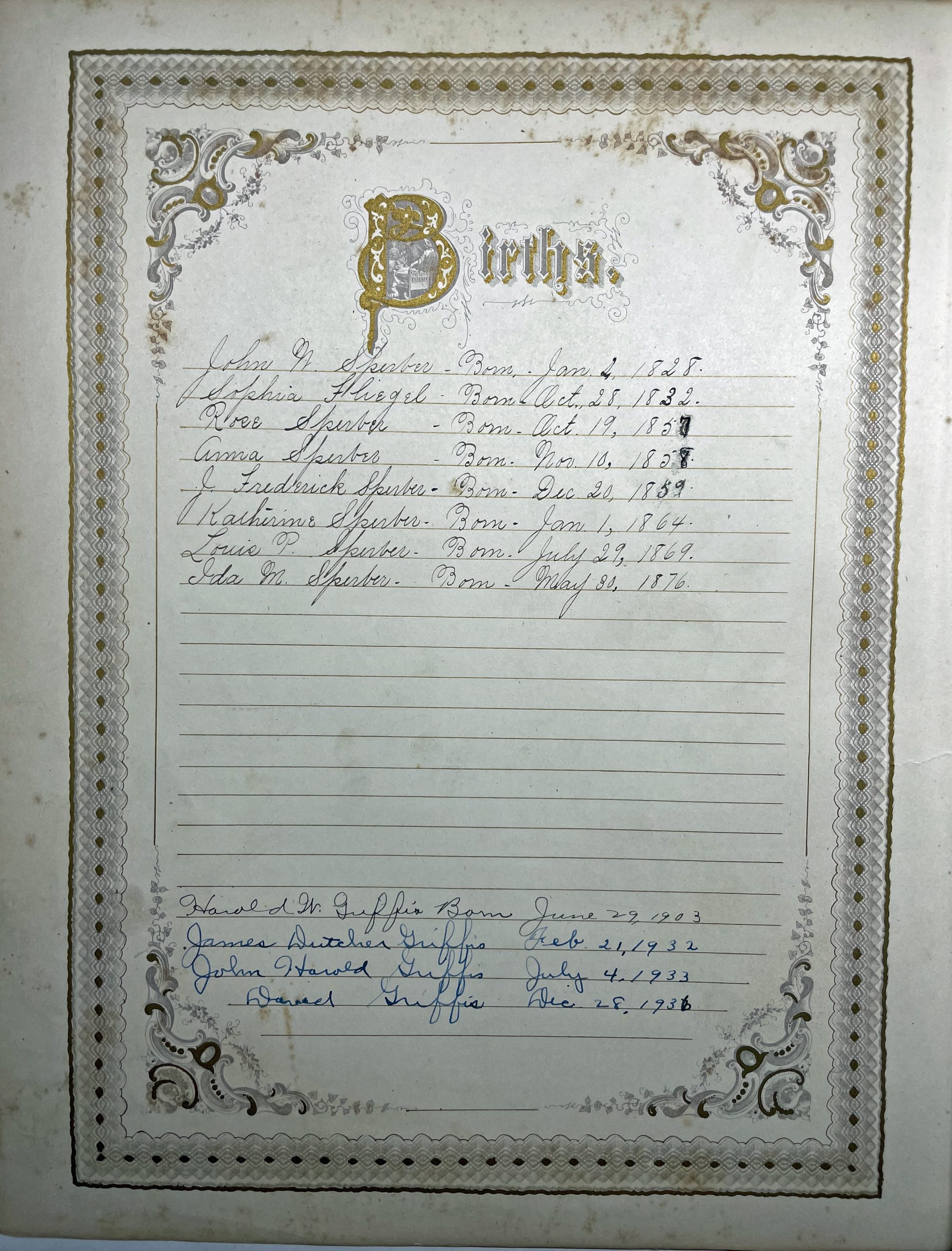
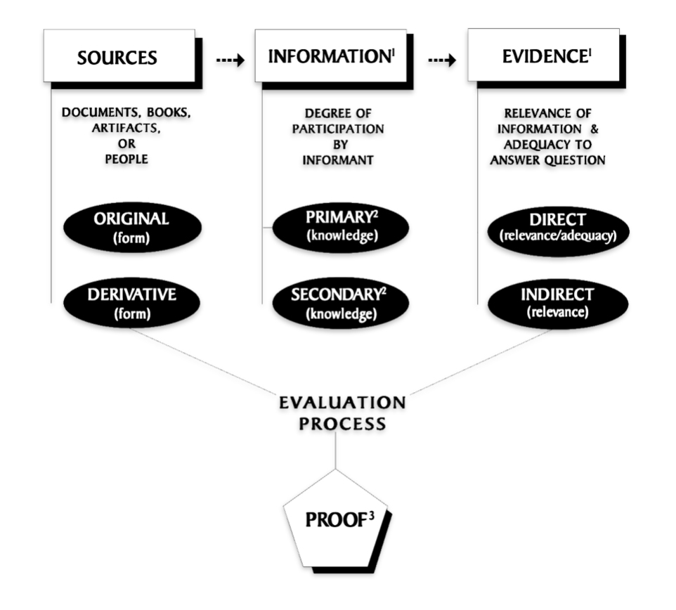
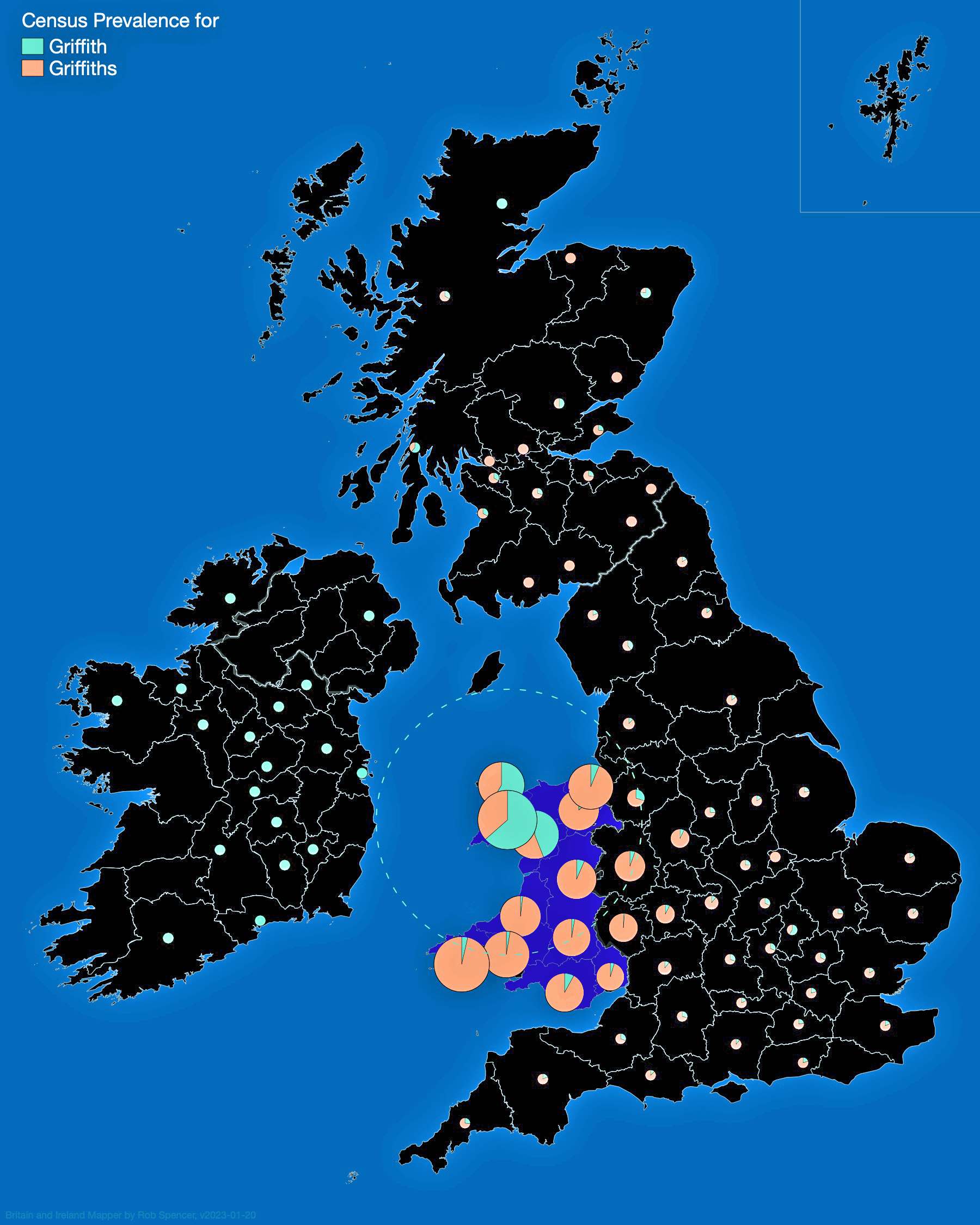
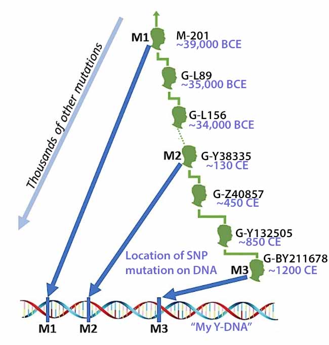