
This story is a continuation of my focus on the G Haplogroup phylogenetic tree of the Griff(is)(es)(ith) patrilineal line of descent and the migratory route of the Griffis family Y-DNA in the long term genealogical time layer.
This part of the story focuses on possible macro social-cultural and enviromental influences that limited the growth of YDNA subclades in the migratory path for one of the two major migratory gaps in the family genetic patrilineal line.
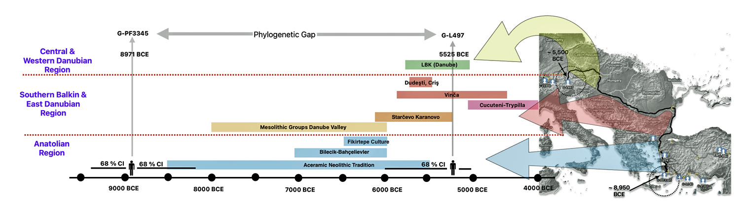
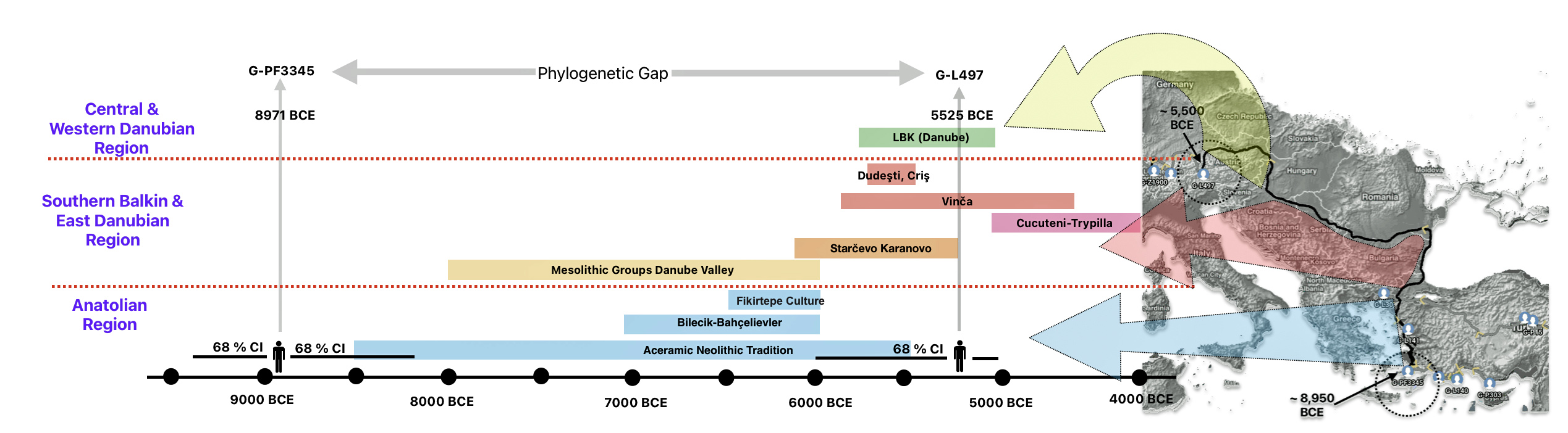
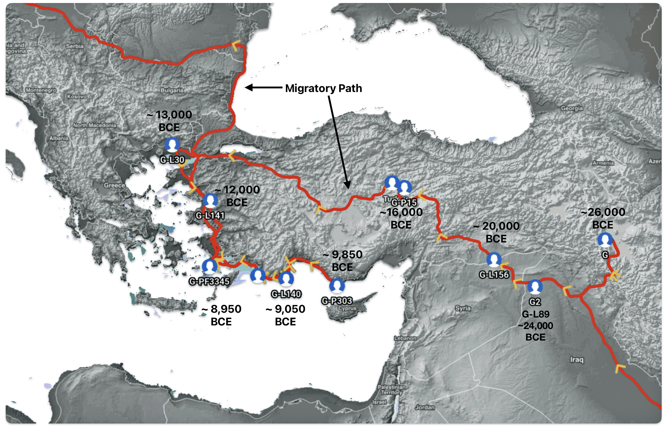
The 3,450 year Gap between G-PF3345 and G-L497: The common ancestor associated with the haplogroup G-PF3345 was born around 8550 Before Common Era (BCE). The next common ancestor in my YDNA line was associated with the G-L497 haplogroup who was born about 3,500 years later, around 5525 BCE. If we use 30 years as an estimate of a generation, this gap between major YDNA mutations represents about 115 generations. (See illustration one.)
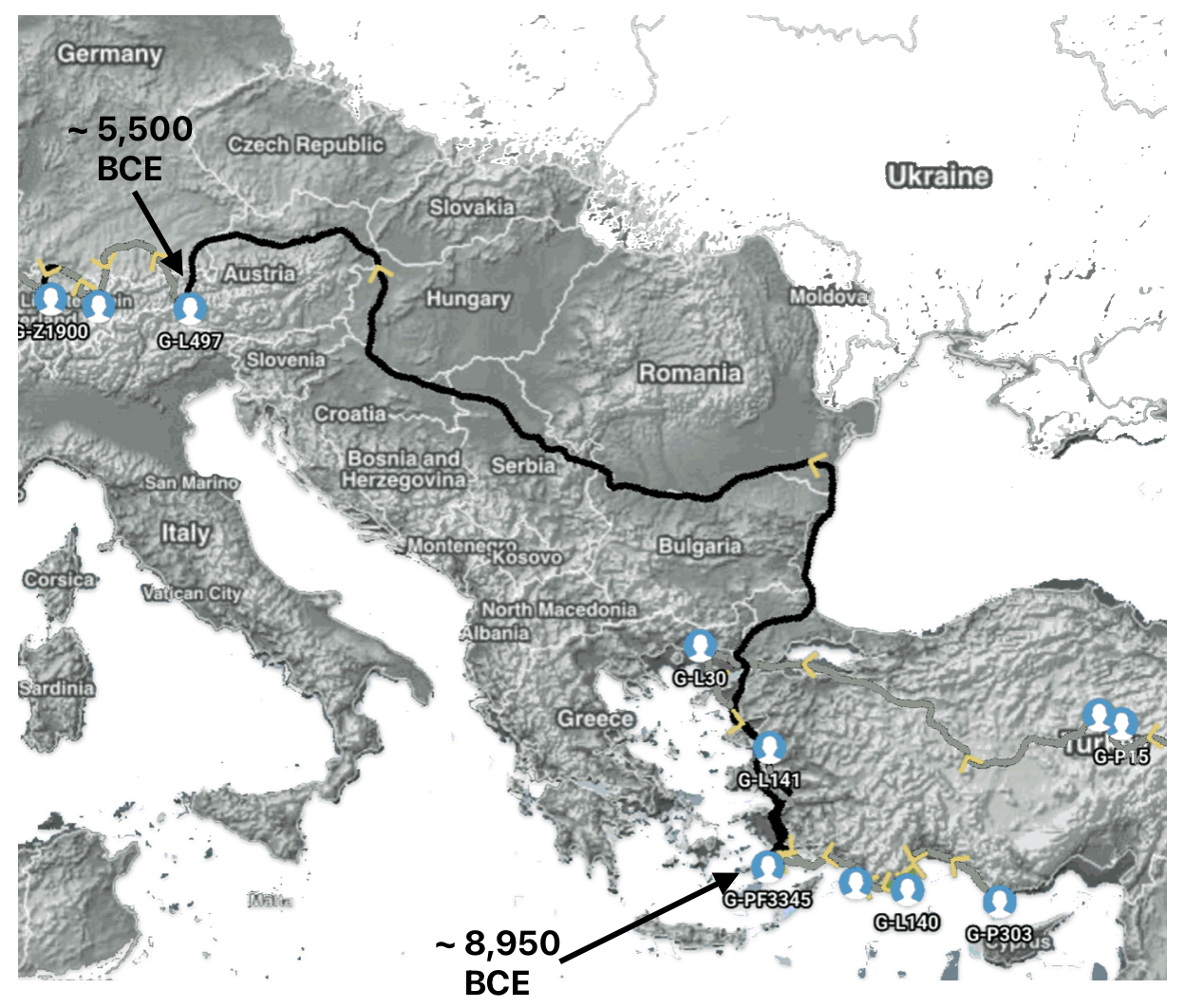
This phylogenetic gap between haplogroup G-PF3345 and G-L497 represents two endpoints in the migratory route that mirrors the ‘continental migratory route‘ of the Early European Farmers from Anatolia to central Europe. (See illustration one.) The migratory northwestern path between the G-PF3345 and G-L497 essentially followed the Danube River which provided a transport route for generations along a river valley that provided fertile, wind-deposited soils that supported intensive cereal cultivation.
Illustration One: The G-PF3345 – G-L497 Phylogenetic Gap
Aside from the methodological factors that may explain the lack of identififed haplogroups in each of these gaps, as outlined in part two of this story, the absence of identified haplogroups in each of these phylogenetic gaps could also be attributed to cultural, social, demographic and environmental influences and factors.
The Migratory Path of the Phylogenetic Gap Between Haplogroups G-PF3345 and G-L497
Haplogroup G-PF3345 (also known as G2a2b2a1a1) is a significant Y-chromosome haplogroup or YDNA ancestor that represents a majority of haplogroup G descendants in modern Europe. Its origins can be traced to the Neolithic and Chalcolithic periods. [1] . While many ancient G subclades disappeared, G-PF3345 became a dominant surviving lineage in European populations. The common ancestor associated with the defining G-PF3345 Y-DNA SNP mutations lived in the Mesolithic Anatolian area. [2]
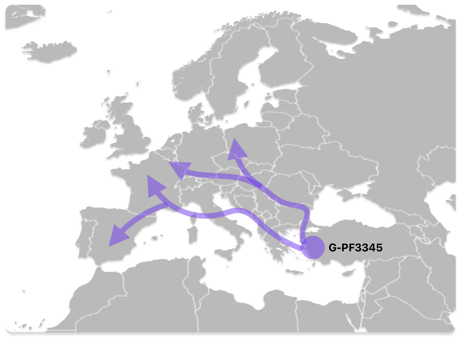
The G-PF3345 haplogroup spread across Europe through both Continental and Mediterranean routes during the Neolithic expansion, as evidenced by ancient DNA and modern distribution patterns. G-PF3345 descendants utilized both routes, with the continental Danubian path shaping Central Europe and the Mediterranean coastal path influencing southern Europe. (See illustration two.)
Illustration Two: Migratory Routes of Descendants of G-PF3345
The Danubian/Continental Route was associated with a number of Neolithic cultures as the G haplogroup made their way along the Danube River. At the ‘tailend’ of this phylogenetic gap, the Linear Pottery (LBK) culture had a notable presence. This path followed the contours of Danube River and its tributaries into Central Europe (~5,500–4,500 BCE). Farmers settled in regions like Germany, Hungary, and Romania, leaving a genetic legacy in modern populations of Austria, Switzerland, and the Czech Republic. [3]
“G2a farmers from the Thessalian Neolithic quickly expanded across the Balkans and the Danubian basin, reaching Serbia, Hungary and Romania by 5800 BCE, Germany by 5500 BCE, and Belgium and northern France by 5200 BCE. Ancient skeletons from the Starčevo–Kőrös–Criș culture (6000-4500 BCE) in Hungary and Croatia, and the Linear Pottery culture (5500-4500 BCE) in Hungary and Germany, all confirmed that G2a (both G2a2a and G2a2b) remained the principal paternal lineage even after farmers intermingled with indigenous populations as they advanced.” [4]
The Mediterranean/Coastal Route was linked to the Cardium Pottery culture, this coastal migration moved westward via the Mediterranean (~5,000 BCE), colonizing Italy, southern France, Iberia, and islands like Sardinia and Corsica.
“These people crossed the Aegean by boat and colonized the Italian peninsula, the Illyrian coast, southern France and Iberia, where they established the Cardium Pottery culture (5000-1500 BCE). Once again, ancient DNA yielded a majority of G2a samples in the Cardium Pottery culture, with G2a frequencies above 80% (against 50% in Central and Southeast Europe).” [5]
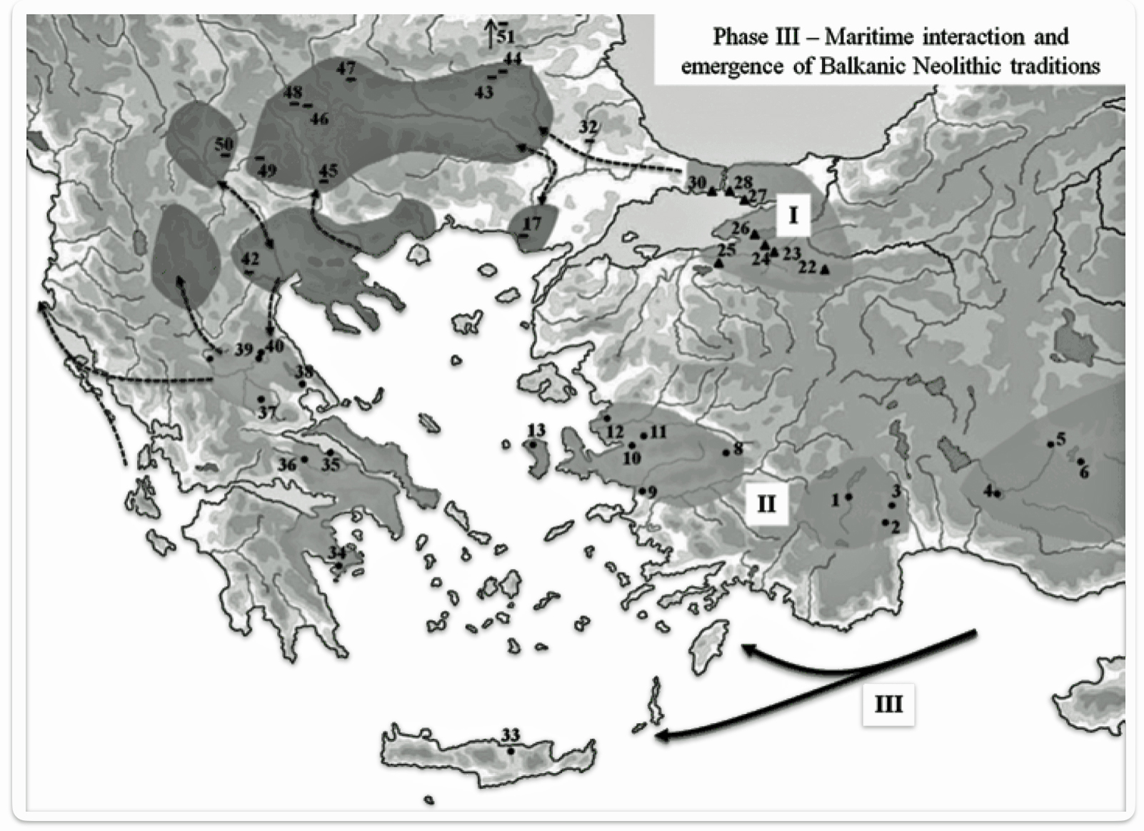
Illustration four provides a map of the Near East and Neolithic Europe. The colored areas represent different Neolithic cultures. The black solid lines represent the areas where estimated cultural and chronological distinctions occurred based on archealogical research. The dotted lines encircle the areas associated with each of the two migrator routes. [6]
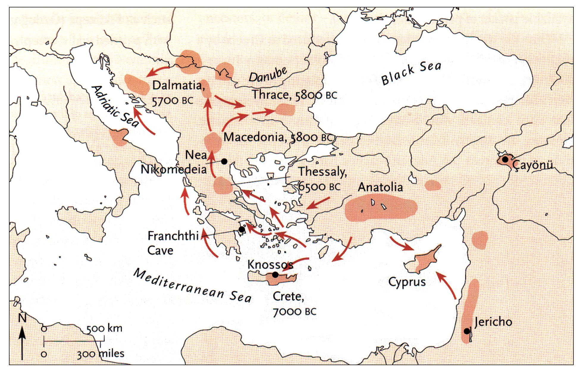
Illustration Four: European Neolithic Cultures Associated with Continental and Mediterranean Migration Routes
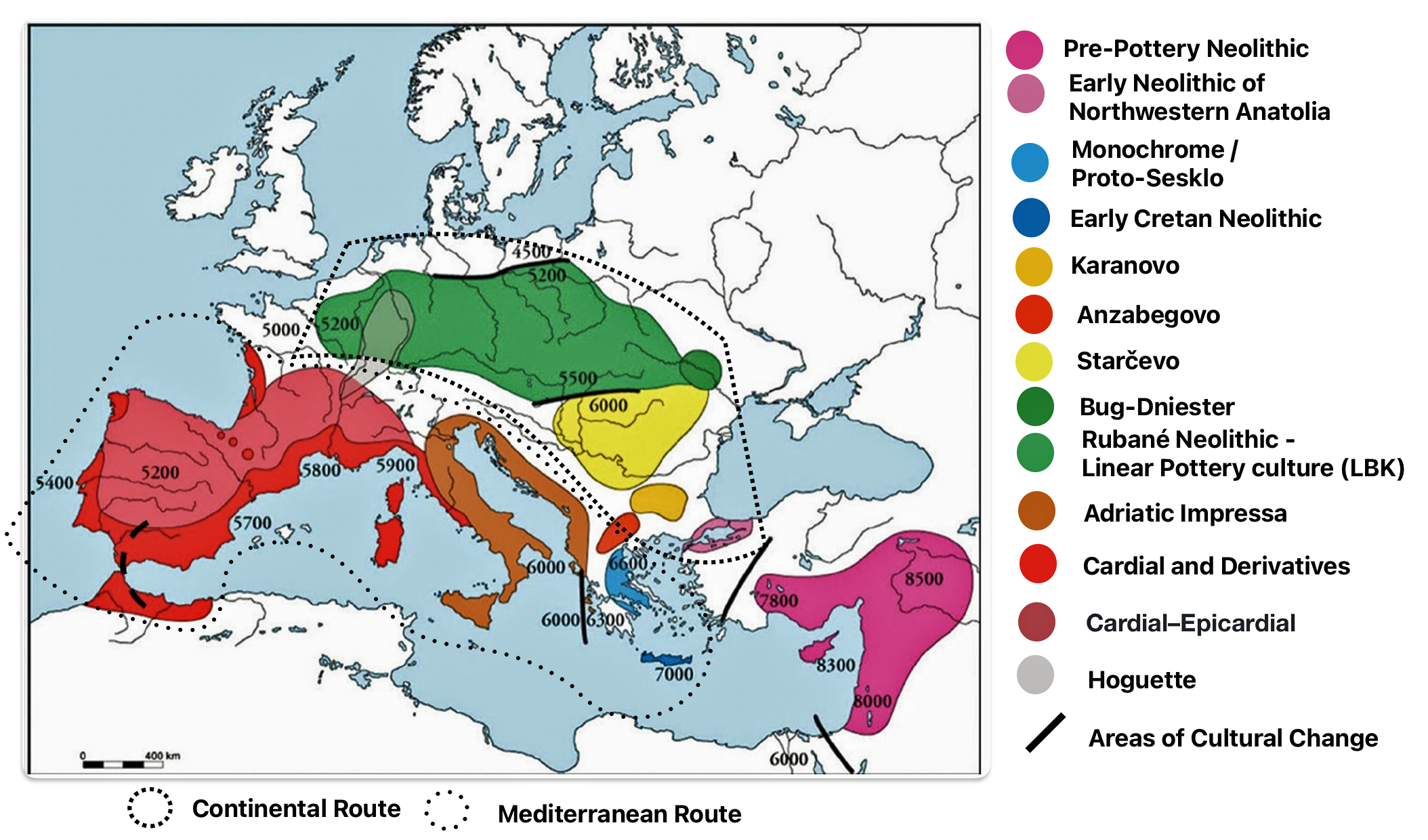
The continental migratory route started northward from Western Anatolia through Greece, and the Southern Balkans (Thrace and Macedonia). [7] The route from Anatolia may have been through settlements of cultures like Karanovo, Hamangia, and Vinčaof, what later became the communities of the LBK (Linear Pottery Culture). The migratory route continued along the Danube River. [8]
The Neolithic Revolution began in the Levant and Anatolia, where domestication of crops like wheat, barley, and legumes, alongside animals such as sheep and goats, laid the foundation for sedentary lifestyles. [9] By 7000 BCE, these practices spread northwestward into southeastern Europe, marking the start of the Continental Route, establishing agro-pastoral communities that later influenced the LBK. [10]
The Anatolian farmers’ migration expansion on the continental route was estimated to be ~0.9 km/year through the Balkans and Central Europe, moving ~50 km per generation. This was slower than the expansion rate associated with the mediterranean route. The continental rate reflects shorter dispersal distances and gradual inland expansion.
A review of various studies on Neolithic expansion indicate the migration of the descendants of the Neolithic Farmers expanded across Europe at an average rate of 1 to 1.3 kilometers per year. This expansion led them to reach the Rhine Valley by around 5300 BCE. [11]
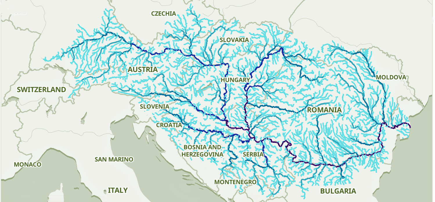
The Danube River is approximately 2,850 kilometers (1,770 miles) long and is part of an extensive water shed (see illustration five). [12] This extensive watershed was the foundation for the Neolithic migration of the G haplogroup into central Europe (see illustration five).
If the estimated expansion rate for the G haplogroup along the Danube River took about 1 to 1.3 km/year, it is conceivable that the it took about 2,565 to 3,700 years to travel the course of the river through successive settlements. The 3,450 year phylogenetic gap coincides with this estimate range of migration expansion.
Illustration Five: The Danube and its Tributaries
The second migratory route, the Southern (Maritime) Route, migrated westward along the coastlines of the Adriatic and Mediterranean Seas. They likely used boats and followed the coastlines, establishing settlements along the way. They reached the Paris Basin by around 5000 BCE. According to some studies, the coastal spread was nearly twice as fast (~1.6 km/year), with farmers traveling ~70 km per generation compared to ~50 km per generation for the contnental route. In the West Mediterranean, rates exceeded 5 km/year, driven by long-distance maritime voyaging (300–450 km per generation). [13]
The inland route’s slower pace stemmed from overland migration with shorter generational movements, while coastal farmers exploited maritime technology for longer jumps. Coastal dispersal involved leapfrog movements (cabotage), allowing farmers to bypass geographical barriers and establish new settlements rapidly. Simulations show sea travel was essential to explain the West Mediterranean’s rapid spread. [14]
Radiocarbon dates indicate the Neolithic farmers reached Portugal (~2,500 km from the Near East) in ~300 years via the Mediterranean, contrasting with slower continental advances. [15]
The Mediterranean route’s faster spread was enabled by maritime technology and longer dispersal jumps, while the continental route’s slower, steadier progress reflected land-based migration patterns. Both pathways involved similar rates of cultural exchange with hunter-gather haplogroups that resided in Europe, but geographical and behavioral factors shaped distinct genetic and demographic outcomes.
The Mitochondrial haplogroup K (common in early farmers) shows a steeper genetic cline along the continental route compared to the Mediterranean, reflecting differences in dispersal distances. [16] Both routes saw about four percent of farmers interbreeding or acculturating hunter gathering groups per generation. However, the Mediterranean route’s longer coastline led to more cumulative genetic admixture events, resulting in higher hunter gatherer ancestry in regions like Iberia. [17]
Social, Cultural, Demographic and Environmental Explanations of the Gap Between G-PF3345 and G-L497
During this temporal phylogentic gap, Europe experienced significant enviromental and demographic shifts that shaped Y-chromosome diversity in Europe. Between 8000 BCE and 5000 BCE, Europe also underwent transformative social and cultural shifts that profoundly shaped Y-chromosome diversity and subclade formation in YDNA haplogroups.
The lack of subclades in this phylogenetic gap may be attributed to a variety of factors. These factors may have had an independent impact on the G haplogroup at various stages in time. The lack of subclade development was driven by the Neolithic transition to agriculture, the migratory effects on the G haplogroup, the rise of patrilineal social structures, population-demographic movements and climatic changes. The earlier phase of this gap may have involved different mechanisms than those of the later, more socially stratified Neolithic societies.
- Impact of Initial Early Neolithic Dispersal of Farming Communities (9000-7000 BCE)
The early portions of the phylogenetic time gap likely represents a series of genetic founder effects, bottlenecks, and localized extinctions that occurred during the critical early expansion phase of agriculture in the Anatolia, Aegean Greece and Thrace area before the development of the more complex social hierarchies.
The transition from the hunting and food gathering stage of the Palaeolithic and Mesolithic eras to the agriculutral stages of the Neolithic Period was marked by the organization of settlements with a permanent character and the systematic practice of farming and stock-rearing. The Neolithization [18] of western Anatolia and southeastern Europe was a dynamic and multifaceted process, with overlapping and simultaneous waves of expansion over more than 1,000 years.
“The transmission of a Neolithic way of life cannot be reduced to the casual introduction of objects, animals and plants, and to the passive acceptance of these new elements by pre-existing populations. It is an active process, which requires 1. learning new techniques and skills and 2. conforming to a Neolithic mode of thought. Alan Barnard suggests that a foraging lifestyle is, by nature, resilient and resistant to the Neolithic, because foraging ideology differs in almost every aspect to that of farming populations; examples include consumption and saving, decision-making and political hierarchy, universal kinship and degree of kin.“
“Repeated interactions and exchanges between foraging and farming groups operating as two independent units during a phase of availability, leads to a rapid substitution of resources followed by a phase of consolidation.“ [19]
An article by Maxime Brami and Volker Heyd, [20] indicates that the movement of early farming groups in the Anatolia region was not a simple, linear process but involved complex interactions, including maritime pioneer colonization and subsequent adoption of agriculture by indigenous populations in the Balkans and Greece. The article revisits and updates the influential hypothesis proposed by James Mellaart [21] which suggested that the earliest Neolithic communities in Greece and the Balkans shared common origins with those in Western Anatolia.
Brami and Heyd argue for a more nuanced view of the Neolithic expansion, emphasizing regional diversity and the importance of Western Anatolia as a dynamic frontier rather than a mere corridor for migration. The spread of farming included the transfer of both material culture and agricultural practices, such as animal husbandry and early dairy technology. The demographic expansion of farming populations from Anatolia into Europe is now understood to have occurred in stages, with Western Anatolia serving as a pivotal intermediary zone.
Small founder groups would establish settlements in new territories. These small pioneer groups carried limited genetic diversity from the outset. Only certain male lineages would be represented in each pioneering settlement. The early phase of the Neolithic transition would have created numerous opportunities for genetic lineage elimination. The small size of pioneering farming communities, coupled with their vulnerability to environmental stresses and potential conflicts, created conditions where entire Y-chromosome lineages could disappear without leaving archaeological traces.
- The Effects of Boom-and-Bust Population Dynamics at the tail end of this gap
A study by Stephen Shennan and other research colleagues, challenges the assumptions of steady population growth during the Neolithic, highlighting the vulnerability of early farming societies to over-exploitation of local environments. The patterns align with broader Neolithic demographic transitions, where initial agricultural productivity gains were offset by long-term ecological or social strain. The study found no correlation between these demographic fluctuations and known climate events, suggesting endogenous causes like unsustainable resource use, soil depletion, or disease. [22]
The introduction of agriculture in Europe around 8,500 years ago ~6550 BCE, initially led to population booms as farming spread westward and northward. However, regional populations subsequently experienced collapses of 30–60 percent, comparable to the demographic impact of the Black Death, an epidemic that peaked in Europe between 1348 and 1350 CE. [23]
These declines occurred in two distinct waves: the first in Central Europe (~7,500 years ago or ~ 5500 BCE) and the second in Northwest Europe (~6,000 years ago or ~4050 BCE). The first wave of population contraction is around the middle to tail end of the phylogenetic gap that is currently being discussed.
Shennan and his colleagues’ research challenges assumptions of steady population growth during the Neolithic, highlighting the vulnerability of early farming societies to overexploitation of local environments. [24]
- Environmental Effects, Demographic Bottlenecks and Founder Effects
The ‘8.2 kiloyear event’, a rapid and significant global cooling episode, occurred approximately around 6,200 BC. It lasted between 150 and 400 years. Different areas were affected at different times and in different ways, some areas became cooler and drier, some cooler and wetter.
The 8.2 kiloyear (ky) event, played a significant role in shaping Early Neolithic population dynamics in the Central Balkans, as outlined by Porčić and his colleagues. The event likely triggered northward migration of farming communities from the southern Balkans/Anatolia into the Central Balkans around 6250 BC, as they sought more favorable conditions amid climatic stress. [25] The Central Balkins is an area just north of Anatolia where haplogroup G-PF33445 orignated.
This northward migration of Anatolian farmers contributed to the first population surge (~6250–6000 BC), which combined high fertility with incoming groups. The 8.2 ky event’s timing aligns with this phase, suggesting environmental pressures accelerated demographic shifts. A population decrease followed around 6000 BC, reaching a low by 5800 BC. A second growth phase (5800–5600 BCE) emerged, attributed primarily to high fertility, before another decline after 5600 BCE.
In Europe, the event had notable ecological and population impacts, such as forest shifts and reductions in Mesolithic populations. The cooling and drying led to significant ecological shifts. Deciduous forests receded in favor of boreal forests in the Alps, while drought conditions in Iberia promoted fire-resistant vegetation. In northeastern Greece, average winter temperatures dropped by over 4°C, likely due to increased influence of the Siberian High. These changes are corroborated by multi-proxy records from caves and sediment cores across southwestern Europe. The cooling and drying led to significant ecological shifts. Deciduous forests receded in favor of boreal forests in the Alps, while drought conditions in Iberia promoted fire-resistant vegetation. [26]
Archaeological records in the Balkans and the Aegean suggest that the Neolithic advance of farming paused for a couple of centuries, possibly because cooler and drier conditions reduced crop yields and slowed population growth. This pause may have allowed plants introduced from the Fertile Crescent to acclimatize to new conditions before farming resumed. [27]
The research by Porčić and his associates supports the Neolithic Demographic Transition (NDT) theory, linking population growth to agricultural adoption and sedentism. The Central Balkan trends mirror demographic shifts in western and central Europe, reinforcing the role of demography in Neolithic expansion. [28]
The Neolithic Demographic Transition (NDT) refers to the period of rapid population growth that occurred after the adoption of agriculture by prehistoric societies. This transition purportedly marked by increased birth rates and stable or slightly decreased death rates, led to a significant increase in population size in many parts of the world. [29]
Haplogroup G, particularly sub-clades like G2a, is strongly associated with Neolithic migrations from Anatolia into Europe. However, its phylogenetic tree shows long, narrow branches during this period, reflecting limited genetic diversity despite population expansion.
This apparent paradox of the G haplogroup exhibiting limited genetic diversity and the NDT theory’s contention of rapid population growth associated with agricultural practices can be explained by several ‘countervailing’ factors:
- Founder Effects of Agricultural Groups During Migration: Neolithic farmers expanding into Europe likely formed small, pioneering groups carrying subsets of G haplogroup diversity. Repeated founder effects the during northwestward migration could have reduced genetic variation in each new population. For example, similar to my G-PF3455 ancestor, the G2a3a-M406 sub-clade shows distinct expansion timelines in Italy (~8,100 years ago) and Iran (~8,800 years ago), aligning with regional Neolithic settlements. These isolated groups preserved specific lineages rather than diversifying broadly. [30]
- Patrilocal Social Structures: As discussed below, genetic evidence suggests patrilocality (males remaining in their birth communities while females marry in) dominated early farming societies. This practice limited male lineage diversity, as Y-chromosomal lineages like G2a were passed down within localized groups.Despite overall population growth, the effective male population size remained small, amplifying genetic drift and reducing haplogroup branching. [31]
- Rapid Expansion with Limited Subsequent Diversification: The Neolithic expansion occurred quickly along migration routes (e.g., the Mediterranean coast and Danube Valley), favoring the spread of specific G sub-clades like G-P303 and G-L497. Once established, these lineages dominated local populations without significant later divergence. [32]
Population bottleneck events that created major population and YDNA subclade collapses could have happened due to: climate change events like the 8.2 kiloyear event; the movemenet of small groups migrating along the Danube River water shed, pandemic diseases in farming communities; and conflict and displacement along the migration path. [33]
- Cultural Practices and Patrilineal Kinship
Research conducted by Monika Karmin and colleagues presents several significant findings that may partly explain the phylogenetic gap. A key discovery from the study was the documentation of a strong bottleneck in male Y-chromosome lineages dating to the last 10,000 years, which contrasts with stable female mitochondrial DNA (mtDNA) patterns. The researchers hypothesize that this recent bottleneck was caused by cultural changes that affected the variance of reproductive success among males. [34]
Illustration six graphically points to the dramatic reduction of male effective population size (Ne) between roughly 8000 BCE to 3000 BCE. Two encircled areas in illustration eleven graphically identify the growth differences in each of the YDNA and mtDNA graphs in this time period.
Illustration Six: Bottleneck of Y Chromosome Diversity Coincides with a Global Change in Culture
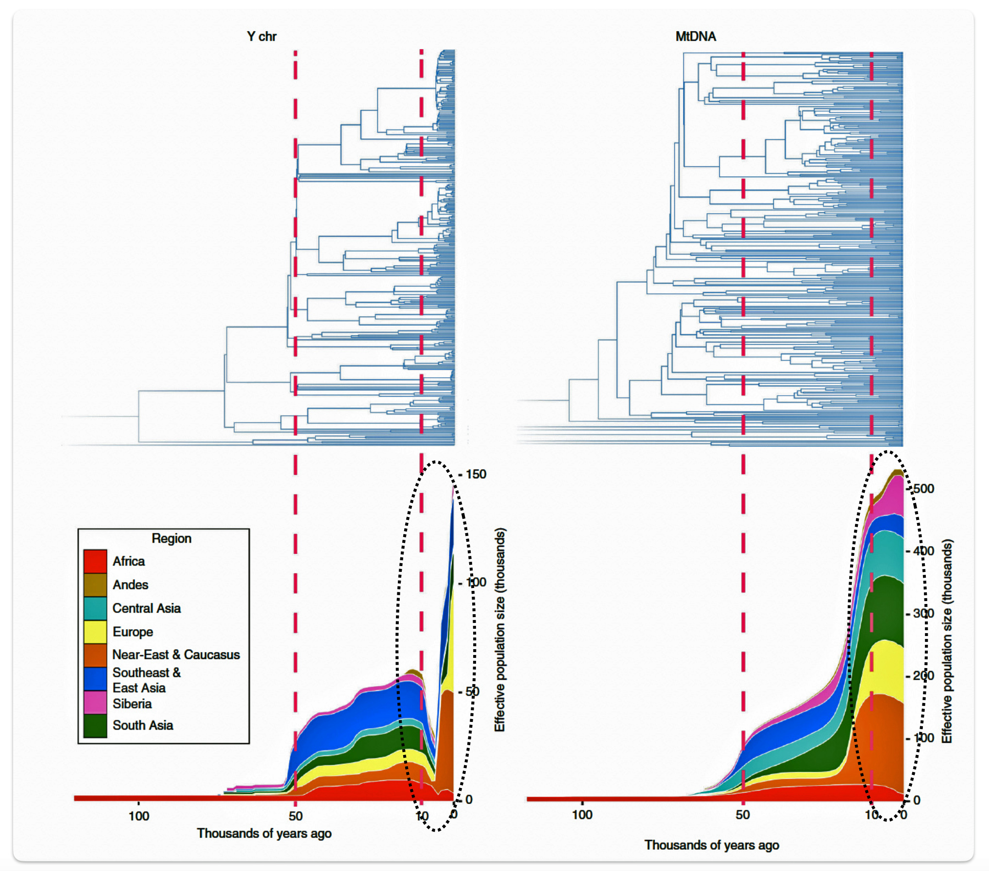
The decline in the male effective population size (Ne) during the Neolithic period was approximately one-twentieth of its original level in various regions of the world. In the same study, mitochondrial sequences indicated a continual increase in population size from the Neolithic to the present, suggesting extreme divergences between the demographic size of male and female populations in the bottleneck period. [35]
The authors of the study suggest the low estimates of male Ne might be explained by culturally driven sex-specific changes in variance in offspring number rather than natural selection. This male-specific decline is attributed to cultural shifts tied to the Neolithic transition to agro-pastoralism, which altered male reproductive variance. This bottleneck coincided with global shifts to agriculture in the Near East and Europe between ~10,500 and 6,500 before present (BP) or between ~ 8550 BCE and 4550 BCE. This coincides with the phylogenetic gap between G-PF3345 and G-L497.
This ‘male altered reproductive variance’ arose through two key mechanisms:
1. Patrilineal Social Systems: The rise of patrilocality (males remaining in birthplace) and patrilineal inheritance (father-to-son wealth/status transmission) concentrated reproductive success among high-status males. This reduced effective male population size while female migration maintained mitochondrial diversity. [36] Ancient DNA from Neolithic/Bronze Age sites shows higher male relatedness (shared Y haplogroups) compared to female diversity, consistent with patrilocal practices. [37]
2. Clan Segmentation and Social Stratification: Patrilineal clans splitting into subclans amplified lineage-specific expansions. Social hierarchies allowed dominant lineages to proliferate, while others dwindled. Models show this process alone—without warfare—could explain the genetic bottleneck. [38]
While initial theories proposed intergroup warfare as the driver of the decline in the male effective population size [39] , subsequent research demonstrated that peaceful patrilineal systems could replicate the bottleneck through:
- Cultural hitchhiking: Y-chromosome lineages became linked to clan identity and success.
- Non-random lineage loss: Clan expansions/extinctions preferentially affected male genetic diversity. [40]
According to the research arguments, this bottleneck coincided with global shifts to agriculture (Near East/Europe: ~10,500–6,500 BP; East Africa/Arabia: ~7,000–5,000 BP), where wealth accumulation incentivized patrilineal inheritance systems. The delayed genetic signal (3,000–5,000 BP) reflects the time required for these social structures to reshape Y-chromosome diversity.
A Look at Anthropological Evidence for Cultural Explanations of the G-PF3345 and G-L497 Gap
Anthropological evidence suggests that Neolithic societies may have practiced patrilocality, where male descendants remained in ancestral territories. This type of social structural practice could suppress lineage diversification by limiting male mobility and reproductive variance. However, it is not a clear-cut case of causation between patrilocality, the increased stratification of wealth and clan segmentation with the reduction of haplgroup subclades.
While specific cultures from western Turkey between 11,000 and 8,000 BCE are not as well documented as in later periods, the region was home to early human groups transitioning from mobile hunter-gatherers to settled, proto-agricultural communities. This period laid the foundation for the more complex Neolithic cultures that would soon flourish across Anatolia. the Aegean and Baltic areas.
Between 9000 BCE and 5000 BCE, which is roughly the time span of the phylogenetic gap, the Danube River region was a cradle of a number of significant prehistoric cultures, transitioning from Mesolithic hunter-gatherers to early Neolithic farming societies. Based on archaeological evidence and scholarly consensus. Below is an overview in illustration seven of the main cultures that existed along the Danube and in the Anatolian and Baltic areas during this period. Depending on the exact and rate of migration, descendants of G-PF3345 could have been part of any of these cultures.
Illustration Seven: Neolithic Cultures that May have been Associated with Griff(is)(es)(ith) ancestors between the Phylogenetic Gap
The ancestor associated with the G-PF3345 haplogroup was born possibly in Western Anatolia during or after the period when human communities transitioned from hunter-gatherer lifestyles to settled agricultural societies. This time frame encompasses the late Epipaleolithic/Mesolithic, Neolithic, and early Chalcolithic periods, representing one of the most transformative eras in human prehistory. Archaeological evidence reveals a diverse cultural landscape with regional variations, technological innovations, and evolving settlement patterns.
The Aceramic Neolithic tradition extended from approximately 8500-5500 BCE across parts of the Middle East, including portions of western Turkey. This period is characterized by permanent settlements, the beginnings of agriculture and animal domestication, but before the widespread adoption of pottery technology. [41]
During this early phase, the spread of Neolithic lifeways appears to have paused in central Anatolia for over a thousand years, only moving westward toward the Aegean after about 7000 BCE. This suggests a period of cultural adaptation and development before further expansion. [42]
The spread of Neolithic farming in the area where the G-PF3345 ancestor lived in Western Anatolia was not a single, rapid event but occurred in at least two definable waves. The first stage was characterized by sparse and sporadic evidence, lasting until around 6500–6400 BC. The second stage was marked by a more substantial and rapid expansion, especially evident in the lakes district and inner western Anatolia. This movement brought with it a “package” of domesticated plants and animals, ground stone artifacts, and building techniques, but left behind most cult and prestige objects, suggesting the migrants were primarily simple farmers or herdsmen. [43]
One of the earliest Neolithic settlements in western Turkey is the Bilecik-Bahçelievler site in northwestern Anatolia, inhabited between approximately 7100 BCE and 6000 BCE. According to radiocarbon dating evidence, this settlement provides some of the earliest results of the Neolithic period in Western Anatolia and offers important information about the beginning and development of the Fikirtepe Culture, which would later become a dominant cultural tradition in the region. [44]
The spread of fully developed Neolithic cultures into western Anatolia became more pronounced after 6500 BCE, with several distinct cultural traditions emerging across the region. The archaeological evidence reveals complex patterns of cultural interaction and regional differentiation across western Turkey during this period. The spread of the Hacılar culture in the south of Western Anatolia and the spread of the Fikirtepe culture in the north is clearly evident. [45]
The Fikirtepe culture represents one of the most significant Neolithic cultural traditions in northwestern Anatolia. Archaeological research has securely placed this culture between 6450 and 6100 BCE. Subsistence was primarily based on farming, with sheep and goat being more common than cattle, and relatively little evidence of hunting compared to earlier periods and other regions. [46]
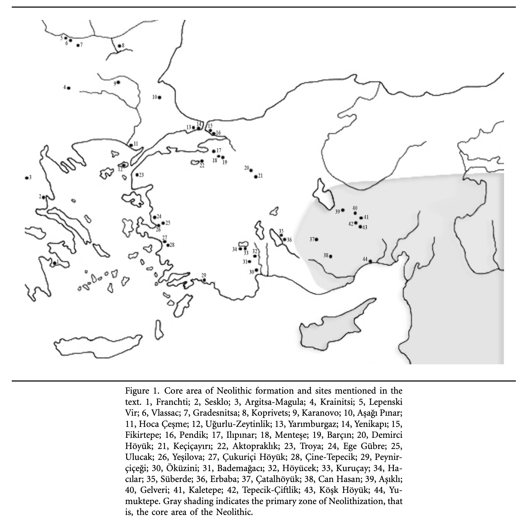
Illustration Eight: Core Areas of Neolitic Formation in Anatolia Region
The archaeological sites in illustration eight correspond with the estimated location of the G-PF3455 haplogroup as well as other G haplogroups identified as part of the Griff(is)(es)(ith) migratory path in the Neolithic era. (see illustration nine.)
Illustration Nine: Location of Early G Haplogroups in Western Asia
A study by Rosenberg and Rocek provides an analysis of Aceramic Neolithic societies in southwestern Asia and challenges traditional assumptions about early social complexity during this time period. Their work emphasizes a complex evolution of socio-political structures, arguing against simplistic models of progression from egalitarian to social hierarchical systems. ‘Heterarchical systems’ prevailed, with multiple overlapping forms of authority (ritual, economic, kinship) rather than centralized hierarchies. Evidence from mega-sites like Göbekli Tepe and Çatalhöyük shows community-based groups coexisting with household-based social structures. [47]
The authors propose that early Neolithic societies developed context-specific solutions to social coordination challenges, blending egalitarian ideals with situational hierarchies. This complexity laid groundwork for later institutionalized inequalities while resisting straightforward categorization into “simple” or “complex” societal types.
Another article by Catherine Twiss and colleagues investigates the nature and extent of social and economic inequality at the Neolithic site of Çatalhöyük in central Anatolia. The study uses a comprehensive, multi-dimensional approach, analyzing a wide range of archaeological data to assess patterns of differentiation among the site’s inhabitants. [48]
The study acknowledges that while some differentiation existed, particularly in symbolic or “prestige” domains, these differences did not amount to entrenched class structures. Çatalhöyük’s society is best characterized as having a “dispersed overlapping mosaic of relationships,” with mechanisms likely in place to suppress or limit the emergence of pronounced hierarchies. Whether the nascent agrarian cultures and social structures in the Aceramic Neolithic societies had an impact on the structure of G haplogroup is not certain.
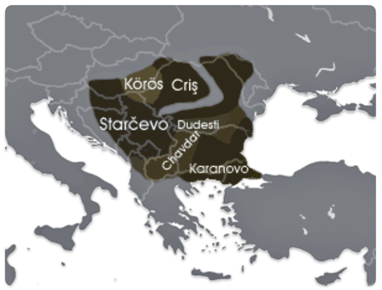
The Neolithic revolution, marked by the adoption of agriculture and settled life, began spreading into the Danube basin from the southeast around 6200–5500 BCE. The Starčevo culture (ca. 6200–5500 BCE) is recognized as the earliest Neolithic culture in the central Danubian region, covering parts of present-day Serbia, Hungary, and Croatia. [49]
In the lower Danube region (modern Bulgaria), the Karanovo culture (ca. 6200–5500 BCE and onward) was another major early Neolithic society, closely related to the spread of farming and settlement patterns in the Balkans. [50] The Dudeşti and Criș Culture in Romania area are contemporaneous with Starčevo and contributed to the Neolithic mosaic along the Danube, particularly in the lower reaches.
Illustration Ten: Extent of the Starčevo–Kőrös–Criș culture (c. 6200-4500 BCE)
After 5000 BCE, the region saw the rise of even more complex societies, such as the Gumelniţa, Cucuteni-Tripolye, and Varna cultures, which are famous for their metallurgy, large settlements, and elaborate burials (see table one and illustration eleven below). [51]
Table One: Neolithic Cultures in the Danube River Valley
| Period | Culture(s) | Location/Extent | Key Features |
|---|---|---|---|
| 8000–6000 BCE | Mesolithic groups | Danube valley (Austria, Hungary, etc.) | Hunter-gatherers, flint tools, fishing, cremation |
| 6200–5500 BCE | Starčevo, Karanovo | Balkans, Central Danube | First farmers, pottery, animal domestication |
| 5500–5000 BCE | LBK (Danubian) | Central/Eastern Europe, Danube basin | Linear pottery, longhouses, intensive agriculture |
| 5700–4500 BCE | Vinča | Middle Danube (Serbia, Balkans) | Large settlements, copper use, early writing |
| ca. 5500 BCE | Dudeşti, Criș | Lower Danube (Romania) | Early Neolithic farming, regional pottery styles |
Illustration Ten: Chalcolithic Cultures of Southeastern Europe with Major Archaeological Sites
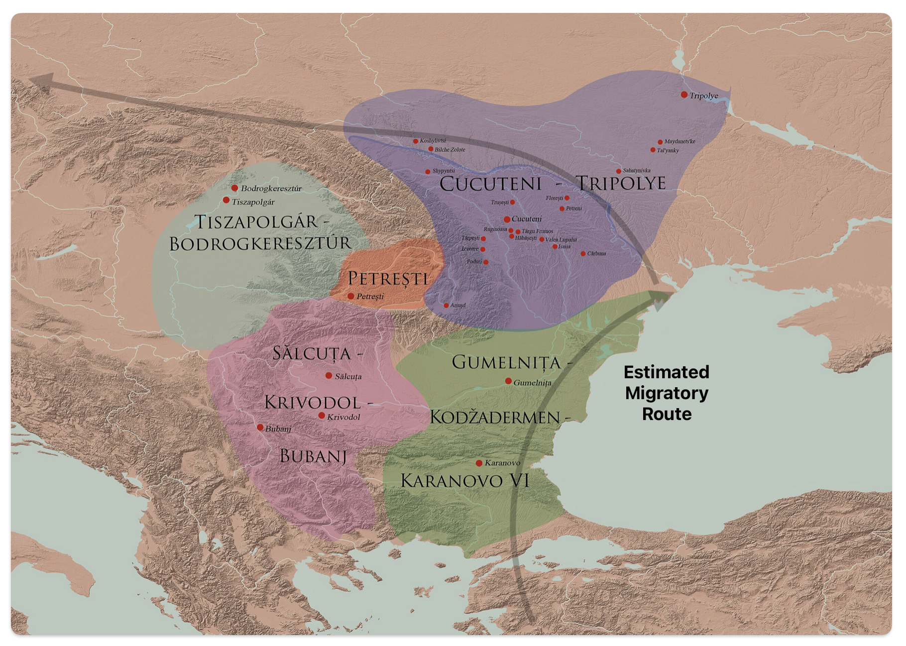
The Cucuteni-Trypillia culture (CTC), linked to G-PF3345, exhibited large, stable settlements that may have reinforced such practices, reducing opportunities for new subclades to emerge and persist. [52]
While the CTC existed during the Y-chromosome bottleneck period, its genetic record does not strongly align with the social or demographic mechanisms driving that bottleneck (e.g., patrilineal kinship, steppe male expansions). CTC settlements show no clear evidence of patrilineal kinship systems—a key driver of the Y-chromosome bottleneck. The culture’s large, planned settlements (e.g., 15,000-resident “mega-sites”) imply collective social organization rather than lineage-based hierarchies. [53]
The culture’s Y-DNA diversity—particularly the persistence of G2a and I2a—suggests it was peripheral to the male-lineage homogenization occurring in steppe-influenced societies. The bottleneck’s primary documentation remains associated with later Indo-European cultures (Steppe), not the CTC. [54]
Researchers have proposed that the formation of patrilineal kin groups and competition between these groups led to a significant reduction in Y-chromosomal diversity through a process called ‘cultural hitchhiking’. In segmentary patrilineal systems, closely related males cluster together in descent groups. Combined with variance in reproductive success between groups, this can substantially reduce Y-chromosome diversity without requiring violence between groups. Patrilineal systems reduced Y diversity within 70–200 generations of their adoption, aligning with Neolithic social changes. [55]
In some societies, particularly after the development of agriculture and herding, a small number of males may have had disproportionate reproductive success, limiting the diversity of YDNA lineages. This social structure could have allowed certain lineages to dominate, potentially eliminating alternative branches that might have otherwise developed into intermediate subclades.
“DNA data suggests dates and places for early PF3345 that correspond with the Neolithic Cucuteni Tripolye culture of Romania and Moldova, with two successful branches developing during the 4th millennium BC -An Eastward expansion (branches of U1) towards the Caucasus and a more general Westward migration towards Southern Germany.” [56]
“The roots of Cucuteni–Trypillia culture can be found in the Starčevo–Körös–Criș and Vinča cultures of the 6th to 5th millennia, with additional influence from the Bug–Dniester culture (6500–5000 BC). During the early period of its existence (in the fifth millennium BC), the Cucuteni–Trypillia culture was also influenced by the Linear Pottery culture from the north, and by the Boian culture from the south.” [57]
As the Griff(is)(es)(ith) patrilineal ancestors migrated westward from the eastern areas of the Danube river, the influences of the of the Linear Pottery culture (LBK) were more evident. [58] The LBK was prominent along the Danube River from approximately 5500 BC to 4500 BC. The culture originated on the middle Danube, particularly in regions of western Hungary, and spread westward along the Danube valley into Central Europe, including present-day Austria, Slovakia, and Germany. This period marks the initial spread of agriculture in Europe, with the LBK representing a major Neolithic horizon in the region. The earliest phase began around 5500 BC, and the culture persisted in various local forms until about 4500 BC. [59]
The LBK shows strong archaeological evidence for patrilocality (males remaining in their birth communities) and patrilineal wealth inheritance, supported by isotopic, genetic, and mortuary analyses. Strontium isotope studies of LBK burials reveal significantly less geographic variance among males compared to females, indicating males typically resided in their birthplace while females migrated from other communities. This pattern aligns with a patrilocal kinship system. [60] Grave goods such as polished adzes, flint tools, and Spondylus shell ornaments disproportionately accompanied male burials, reflecting intergenerational wealth transmission. These items symbolized agricultural authority and social status. [61] Genetic analyses of LBK populations show Y-chromosome haplogroups (e.g., G2a, I2) passed through male lines, consistent with patrilineal descent. Conversely, mitochondrial DNA diversity suggests female exogamy. [62]
LBK longhouses likely housed multigenerational male kin groups, with land and resources controlled patriarchally. [63] The standardization of house architecture and tool traditions over centuries implies stable male-dominated inheritance practices. [64] Empty grave plots in LBK cemeteries may represent symbolic claims to lineage-based land rights, further reinforcing hereditary wealth structures.[65] This evidence collectively underscores a society where male lineage dictated resource access and social standing, with women integrating into new communities through marriage.
Conclusion and the Next Phylogenetic Gap
The Griff(is)(es)(ith) genetic ancestral paternal line was associated with Neolithic migrations from Anatolia into Europe. However, its phylogenetic tree shows long, narrow branches during this transformative historical period, reflecting limited genetic diversity despite the geographical and population expansion of the G haplogroup into central and western Europe.
This limited genetic diversity and lack of documented haplgroups along this migratory path can be explained by several envronmental, demographic, social and cultural ‘countervailing’ factors.
The next and final part of this story on the phyogentic structure of the Griff(is)(es)(ith) genetic ancestral paternal line focuses on the second gap between between G-FGC7516 and G-Z6748.
Source:
Feature Banner: The banner at the top of the story features a map of the phylogenetic gap discussed in the story. The map was generated by taking snapshops from the FamilyTreeDNA GlobetrekkerTM video of the migratory path of my YDNA descendants over time. The map shows the migratory path of selected most common recent ancestors and their respective estimated dates of birth.
[1] The enigma of G-PF3345 (U1, CTS342 and L497), 3 Sep 2018, G2a, YDNA Haplogroups, Population Genetics, Forums, Eupedia, https://www.eupedia.com/forum/threads/the-enigma-of-g-pf3345-u1-cts342-and-l497.37040/
[2] Mares, Boed, G-M201, 19 Feb 2025, Marres, https://www.marres.nl/EN/G-M201.htm
Genetic studies on Croats, Wikipedia, This page was last edited on 10 March 2025, https://en.wikipedia.org/wiki/Genetic_studies_on_Croats
Di Cristofaro J, Mazières S, Tous A, Di Gaetano C, Lin AA, Nebbia P, Piazza A, King RJ, Underhill P, Chiaroni J. Prehistoric migrations through the Mediterranean basin shaped Corsican Y-chromosome diversity. PLoS One. 2018 Aug 1;13(8):e0200641. doi: 10.1371/journal.pone.0200641. PMID: 30067762; PMCID: PMC6070208. (PubMed) https://pmc.ncbi.nlm.nih.gov/articles/PMC6070208/
Your Haplogroup Story: G-PF3345 , FamilyTreeDNA , https://discover.familytreedna.com/y-dna/G-PF3345/story
Linear Pottery culture, Wikipedia, This page was last edited on 3 April 2025, https://en.wikipedia.org/wiki/Linear_Pottery_culture
Danubian culture, Wikipedia, This page was last edited on 15 June 2024, https://en.wikipedia.org/wiki/Danubian_culture
Hay, Maciamo, Linear Pottery (LBK) culture (c. 5600-4250 BCE), Eupedia, https://www.eupedia.com/genetics/linear_pottery_culture.shtml
[3] Fort, J., Pérez-Losada, J. Interbreeding between farmers and hunter-gatherers along the inland and Mediterranean routes of Neolithic spread in Europe. Nat Commun 15, 7032 (2024). https://doi.org/10.1038/s41467-024-51335-4
N. Isern, J. Zilhão, J. Fort, & A.J. Ammerman, Modeling the role of voyaging in the coastal spread of the Early Neolithic in the West Mediterranean, Proc. Natl. Acad. Sci. U.S.A. 114 (5) 897-902, 2017 https://doi.org/10.1073/pnas.1613413114
[4] Hay, Maciamo, Linear Pottery (LBK) culture (c. 5600-4250 BCE), Eupedia, https://www.eupedia.com/genetics/linear_pottery_culture.shtml
[5] Ibid
[6] The name and definition of the color coded areas in the map are below, with references:
Pre-Pottery Neolithic (PPNB) – Pre-Pottery Neolithic B, Wikipedia, This page was last edited on 26 January 2025, https://en.wikipedia.org/wiki/Pre-Pottery_Neolithic_B
Early Neolithic of Northwestern Anatolia – See for example Karul, Necmi. (2022). The Beginning and the Development of Farming-Based Village Life in Northwestern Anatolia / 2022. 231-246. 10.1017/9781107337640.017 https://www.researchgate.net/publication/360398204_The_Beginning_and_the_Development_of_Farming-Based_Village_Life_in_Northwestern_Anatolia_2022
Monochrome / Proto-Sesklo – Sesklo, Wikipedia, This page was last edited on 22 October 2024, https://en.wikipedia.org/wiki/Sesklo
Karanovo – Karanovo culture, Wikipedia, This page was last edited on 23 March 2025, https://en.wikipedia.org/wiki/Karanovo_culture
Anzabegovo – Marco Porcic, Evaluating Social Complexity and Inequality in the Balkans Between 6500 and 4200 BC, Journal of Archaeological Research 27(3):335-390 DOI:10.1007/s10814-018-9126-6, https://www.researchgate.net/publication/327425832_Evaluating_Social_Complexity_and_Inequality_in_the_Balkans_Between_6500_and_4200_BC
Starčevo – Starčevo culture, Wikipedia, This page was last edited on 29 November 2024, https://en.wikipedia.org/wiki/Starčevo_culture
Bug-Dniester Bug – Dniester culture, Wikiedia, This page was last edited on 2 October 2024, https://en.wikipedia.org/wiki/Bug–Dniester_culture
Rubané Neolithic – Linear Pottery culture (LBK), Wikipedia, This page was last edited on 3 April 2025, https://en.wikipedia.org/wiki/Linear_Pottery_culture
Adriatic Impressa- Cardium pottery, Wikipedia, This page was last edited on 24 February 2025, This page was last edited on 24 February 2025, https://en.wikipedia.org/wiki/Cardium_pottery
Cardial and Derivatives – The term “Cardial” refers to a specific pottery style and associated culture of the Early Neolithic period in Southern Europe, particularly along the Mediterranean coast. Cardial pottery is characterized by distinctive impressions, often made using the edges of Cardium shells, and is a key marker of the Cardial culture. Derivatives of Cardial, such as Epicardial, represent later developments or variations within the Cardial tradition. See Cardium pottery, Wikipedia, This page was last edited on 24 February 2025, This page was last edited on 24 February 2025, https://en.wikipedia.org/wiki/Cardium_pottery
Epicardial – Elsa Defranould. The Cardial–Epicardial Early Neolithic of Lower Rhône Valley (South-Eastern France): A Lithic Perspective. Open Archaeology, 2021, 7 (1), pp.939-952. ⟨10.1515/opar-2020-0182⟩. ⟨hal-04913839⟩. https://hal.science/hal-04913839
Hoguette – La Hoguette, Wikipedia, This page was last edited on 15 April 2025, https://en.wikipedia.org/wiki/La_Hoguette
[7] Thrace refers to a historical region in Southeast Europe, now divided between Bulgaria, Greece, and Turkey. Thrace today is divided among three modern nations: southeastern Bulgaria (Northern Thrace), northeastern Greece (Western Thrace), and the European part of Turkey (East Thrace). The historical region of Thrace encompassed these areas and more, extending along the Balkan Peninsula.
Macedonia refers to both a historical region and a modern country in Southeastern Europe. Historically, it encompasses an area including parts of Greece, Bulgaria, and the modern-day Republic of North Macedonia. The Republic of North Macedonia, formerly known as the Republic of Macedonia, is a landlocked country with a diverse history and culture, bordering Greece, Albania, Bulgaria, Kosovo, and Serbia.
Macedonia, Wikipedia, This page was last edited on 30 April 2025, https://en.wikipedia.org/wiki/Macedonia
Thracia, Wikipedia, This page was last edited on 28 January 2025, https://en.wikipedia.org/wiki/Thracia
Thrace, Wikipedia, This page was last edited on 24 March 2025, https://en.wikipedia.org/wiki/Thrace
[8] Neolithic Revolution, Wikipedia, This page was last edited on 16 April 2025, https://en.wikipedia.org/wiki/Neolithic_Revolution
[9] Neolithic, Wikipedia, This page was last edited on 26 April 2025, https://en.wikipedia.org/wiki/Neolithic
[10] Szécsényi-Nagy A, Brandt G, Haak W, Keerl V, Jakucs J, Möller-Rieker S, Köhler K, Mende BG, Oross K, Marton T, Osztás A, Kiss V, Fecher M, Pálfi G, Molnár E, Sebők K, Czene A, Paluch T, Šlaus M, Novak M, Pećina-Šlaus N, Ősz B, Voicsek V, Somogyi K, Tóth G, Kromer B, Bánffy E, Alt KW. Tracing the genetic origin of Europe’s first farmers reveals insights into their social organization. Proc Biol Sci. 2015 Apr 22;282(1805):20150339. doi: 10.1098/rspb.2015.0339. PMID: 25808890; PMCID: PMC4389623, (PubMed) https://pmc.ncbi.nlm.nih.gov/articles/PMC4389623/
Szécsényi-Nagy A, et al, Tracing the genetic origin of Europe’s first farmers reveals insights into their social organization, 22 April 2015, Proceedings of the Royal Society Biological, https://doi.org/10.1098/rspb.2015.0339, https://royalsocietypublishing.org/doi/10.1098/rspb.2015.0339
[11] Fort, J., Pérez-Losada, J. Interbreeding between farmers and hunter-gatherers along the inland and Mediterranean routes of Neolithic spread in Europe. Nat Commun 15, 7032 (2024). https://doi.org/10.1038/s41467-024-51335-4
Pinhasi, Ron, Joaquin Fort, Albert J Ammerman, Tracing the Origin and Spread of Agriculture in Europe, 29 Nov 2005, PLOS, https://doi.org/10.1371/journal.pbio.0030410
Alexandros Tsoupas, Carlos S. Reyna-Blanco, Claudio S. Quilodrán, Jens Blöcher, Maxime Brami, Daniel Wegmann, Joachim Burger, Mathias Currat, Local increases in admixture with hunter-gatherers followed the initial expansion of Neolithic farmers across continental Europe, bioRxiv, 12 Jun 2024, doi: https://doi.org/10.1101/2024.06.10.598301 , https://www.biorxiv.org/content/10.1101/2024.06.10.598301v1.full.pdf
[12] Danube River Map, Atlas, https://atlas.co/explore/rivers/danube-river/
[13] N. Isern, J. Zilhão, J. Fort, & A.J. Ammerman, Modeling the role of voyaging in the coastal spread of the Early Neolithic in the West Mediterranean, Proc. Natl. Acad. Sci. U.S.A. 114 (5) 897-902, 2017, https://doi.org/10.1073/pnas.1613413114 .
Fort, J., Pérez-Losada, J. Interbreeding between farmers and hunter-gatherers along the inland and Mediterranean routes of Neolithic spread in Europe. Nat Commun 15, 7032 (2024). https://doi.org/10.1038/s41467-024-51335-4
Neolithic Revolution, Wikipedia, This page was last edited on 16 April 2025, https://en.wikipedia.org/wiki/Neolithic_Revolution
By comparing Neolithic spread rates in several regions of the world, Joaquim Fort proposed the following ‘ laws of Neolithic Expansion’:
- The Neolithic spread inland at a rate of about 1 km/yr, but there was substantial variation (0.44-3.6 km/yr)
- When in addition to demic diffusion there is substantial cultural diffusion, Neolithic spread rates are faster.
- Neolithic spread rates over the sea take place at about 10 km/yr.
- Most inland and coastal Neolithic spreads were mainly demic.
- Neolithic spread rates tend to become slower at higher latitudes.
- The Neolithic spreads later and more slowly at higher altitudes above sea level (compared to surrounding regions). A spatial interpolation of early Neolithic dates in Europe has made it possible to map the isochrones every 250 years and this has shown that the Neolithic first surrounded the Alps completely, and only later begun to climb up these mountains
Fort, Joaquim, Prehistoric spread rates and genetic clines, 6 Apr 2022, Human Population Genetic and Genomics, 2022; 2(2):0003, https://www.pivotscipub.com/hpgg/2/2/0003
See also:
Aoki, Kenici, Interpreting the demic diffusion of early farming in Europe with a three-population model , 8 Oct 2024 ,Human Population Genetics and Genomics, 2024;4(4):0010, https://doi.org/10.47248/hpgg2404040010
Michael Kempf, Solène Denis, Resource dependency and communication networks in Early Neolithic western Europe, Quaternary Environments and Humans,
Volume 2, Issue 5, 2024, 100014, ISSN 2950-2365, https://doi.org/10.1016/j.qeh.2024.100014 .
(https://www.sciencedirect.com/science/article/pii/S2950236524000124 )
Marko Porčića,Tamara Blagojević, Jugoslav Pendić,Sofija Stefanović, The timing and tempo of the Neolithic expansion across the Central Balkans in the light of the new radiocarbon evidence, Journal of Archaeological Science: Reports, Vol 33, Oct 2020, 102528, 1 – 12, https://www.sciencedirect.com/science/article/pii/S2352409X20303199
Peter Rowley-Conwy, Westward Ho! The Spread of Agriculture from Central Europe to the Atlantic, Current Anthropology Volume
[14] N. Isern, J. Zilhão, J. Fort, & A.J. Ammerman, Modeling the role of voyaging in the coastal spread of the Early Neolithic in the West Mediterranean, Proc. Natl. Acad. Sci. U.S.A. 114 (5) 897-902, 2017, https://doi.org/10.1073/pnas.1613413114 .
Paschou P, Drineas P, Yannaki E, Razou A, Kanaki K, Tsetsos F, Padmanabhuni SS, Michalodimitrakis M, Renda MC, Pavlovic S, Anagnostopoulos A, Stamatoyannopoulos JA, Kidd KK, Stamatoyannopoulos G. Maritime route of colonization of Europe. Proc Natl Acad Sci U S A. 2014 Jun 24;111(25):9211-6. doi: 10.1073/pnas.1320811111. Epub 2014 Jun 9. PMID: 24927591; PMCID: PMC4078858, (PubMed) https://pmc.ncbi.nlm.nih.gov/articles/PMC4078858/
[15] N. Isern, J. Zilhão, J. Fort, & A.J. Ammerman, Modeling the role of voyaging in the coastal spread of the Early Neolithic in the West Mediterranean, Proc. Natl. Acad. Sci. U.S.A. 114 (5) 897-902 2017, ,https://doi.org/10.1073/pnas.1613413114
Paschou P, et al, Maritime route of colonization of Europe. Proc Natl Acad Sci U S A. 2014 Jun 24;111(25):9211-6. doi: 10.1073/pnas.1320811111. Epub 2014 Jun 9. PMID: 24927591; PMCID: PMC4078858, (PubMed) https://pmc.ncbi.nlm.nih.gov/articles/PMC4078858/
[16] Fort, J., Pérez-Losada, J. Interbreeding between farmers and hunter-gatherers along the inland and Mediterranean routes of Neolithic spread in Europe. Nat Commun 15, 7032 (2024). https://doi.org/10.1038/s41467-024-51335-4
[17] Fort, J., Pérez-Losada, J. Interbreeding between farmers and hunter-gatherers along the inland and Mediterranean routes of Neolithic spread in Europe. Nat Commun 15, 7032 (2024). https://doi.org/10.1038/s41467-024-51335-4
Alexandros Tsoupas, Carlos S. Reyna-Blanco, Claudio S. Quilodrán, Jens Blöcher, Maxime Brami, Daniel Wegmann, Joachim Burger, Mathias Currat, Local increases in admixture with hunter-gatherers followed the initial expansion of Neolithic farmers across continental Europe, bioRxiv, 12 Jun 2024, doi: https://doi.org/10.1101/2024.06.10.598301 , https://www.biorxiv.org/content/10.1101/2024.06.10.598301v1.full.pdf
Paschou P, Drineas P, Yannaki E, Razou A, Kanaki K, Tsetsos F, Padmanabhuni SS, Michalodimitrakis M, Renda MC, Pavlovic S, Anagnostopoulos A, Stamatoyannopoulos JA, Kidd KK, Stamatoyannopoulos G. Maritime route of colonization of Europe. Proc Natl Acad Sci U S A. 2014 Jun 24;111(25):9211-6. doi: 10.1073/pnas.1320811111. Epub 2014 Jun 9. PMID: 24927591; PMCID: PMC4078858 (PubMed) https://pmc.ncbi.nlm.nih.gov/articles/PMC4078858/
Szécsényi-Nagy A, et al, Tracing the genetic origin of Europe’s first farmers reveals insights into their social organization, 22 April 2015, Proceedings of the Royal Society Biological, https://doi.org/10.1098/rspb.2015.0339, https://royalsocietypublishing.org/doi/10.1098/rspb.2015.0339
Maïté Rivollat et al. , Ancient genome-wide DNA from France highlights the complexity of interactions between Mesolithic hunter-gatherers and Neolithic farmers.Sci. Adv.6,eaaz5344(2020).DOI:10.1126/sciadv.aaz5344
e 52, Supplement 4, October 2011, S431-451, https://www.journals.uchicago.edu/doi/epdf/10.1086/65836
[18] Neolithization refers to the process of a society transitioning from a hunter-gatherer lifestyle to a settled agricultural one, marking the transition to the Neolithic period. It essentially describes the widespread adoption of farming and the establishment of villages, signifying a fundamental shift in human societies.
Goce Naumov, The Early Neolithic communities in Macedonia, Archeologické rozhledy LXVII–2015, 331-355 , DOI: 10.35686/AR.2015.18, https://www.researchgate.net/publication/292392154
See also Todd Paradine, Haplogroup G in the New Stone Age, April 2021, GM3302, https://sites.google.com/view/gm3302/the-story/neolithic; PDF verson
[19] Maxime Brami and Volker Heyd, The origins of Europe’s first farmers: The role of Hacılar and Western Anatolia, fifty years on, Oct 2011, Praehistorische Zeitschrift 86(2) 193, DOI: 10.1515/pz.2011.011
[20] Maxime Brami and Volker Heyd, The origins of Europe’s first farmers: The role of Hacılar and Western Anatolia, fifty years on, Oct 2011, Praehistorische Zeitschrift 86(2)165-206, DOI: 10.1515/pz.2011.011
See also M. Brami, ‘Aegean’ and ‘Anatolian’ first farmers: ambiguous labelling or research blind spot. In: A. Lahelma, M. Ahola, E. Holmqvist-Sipilä, K. Mannermaa, K. Nordqvist eds., Moving northward: Professor Volker Heyd’s Festschrift as he turns 60 (Archaeological Society of Finland) 209-219 https://www.academia.edu/106735707/_2023_M_Brami_Aegean_and_Anatolian_first_farmers_ambiguous_labelling_or_research_blind_spot_In_A_Lahelma_M_Ahola_E_Holmqvist_Sipilä_K_Mannermaa_K_Nordqvist_eds_Moving_northward_Professor_Volker_Heyds_Festschrift_as_he_turns_60_Archaeological_Society_of_Finland_209_219
[21] Mellaart, James, Excavations at Hacılar: Third Preliminary Report, Anatolian Stud. 10, 1960, 83–104
Mellaart, James, Excavations at Halicar, Edinburgh, Published for British Institute of Archaeology at Ankara. Edinburgh University Press, 1970 https://archive.org/details/excavationsathac0002mell/page/n3/mode/2up
See also Shennan S. The Origins of Agriculture in South-West Asia. In: The First Farmers of Europe: An Evolutionary Perspective. Cambridge World Archaeology. Cambridge University Press; 2018:16-54.
[22] Shennan S, Downey SS, Timpson A, Edinborough K, Colledge S, Kerig T, Manning K, Thomas MG. Regional population collapse followed initial agriculture booms in mid-Holocene Europe. Nat Commun. 2013;4:2486. doi: 10.1038/ncomms3486. PMID: 24084891; PMCID: PMC3806351, (PubMed) https://pubmed.ncbi.nlm.nih.gov/24084891/
Bower, Bruce, Ancient farming populations went boom, then bust, 1 Oct 2013, Science News, https://www.sciencenews.org/article/ancient-farming-populations-went-boom-then-bust
[23] Porčić Marko, Blagojević Tamara, Pendić Jugoslav and Stefanović Sofija, The Neolithic Demographic Transition in the Central Balkans: population dynamics reconstruction based on new radiocarbon evidence Phil. Trans. R. Soc. 30 Nov 2020, B37620190712 http://doi.org/10.1098/rstb.2019.0712
[24] Shennan S, Downey SS, Timpson A, Edinborough K, Colledge S, Kerig T, Manning K, Thomas MG. Regional population collapse followed initial agriculture booms in mid-Holocene Europe. Nat Commun. 2013;4:2486. doi: 10.1038/ncomms3486. PMID: 24084891; PMCID: PMC3806351, (PubMed) https://pubmed.ncbi.nlm.nih.gov/24084891/
Bower, Bruce, Ancient farming populations went boom, then bust, 1 Oct 2013, Science News, https://www.sciencenews.org/article/ancient-farming-populations-went-boom-then-bust
[25] Porčić Marko, et al, The Neolithic Demographic Transition in the Central Balkans: population dynamics reconstruction based on new radiocarbon evidence Phil. Trans. R. Soc. 30 Nov 2020, B37620190712 http://doi.org/10.1098/rstb.2019.0712
[26] 8.2-kiloyear event, Wikipedia, This page was last edited on 28 March 2025, https://en.wikipedia.org/wiki/8.2-kiloyear_event
García-Escárzaga A, Gutiérrez-Zugasti I, Marín-Arroyo AB, Fernandes R, Núñez de la Fuente S, Cuenca-Solana D, Iriarte E, Simões C, Martín-Chivelet J, González-Morales MR, Roberts P. Human forager response to abrupt climate change at 8.2 ka on the Atlantic coast of Europe. Sci Rep. 2022 Apr 20;12(1):6481. doi: 10.1038/s41598-022-10135-w. PMID: 35444222; PMCID: PMC9021199, (PubMed) https://pmc.ncbi.nlm.nih.gov/articles/PMC9021199/
King, David T., 8.2 kiloyear event, 2025, EBSCO, https://www.ebsco.com/research-starters/earth-and-atmospheric-sciences/82-kiloyear-event
Dixit, Y., Chua, S., Yan, Y.T. et al. Hydroclimatic impacts of the abrupt cooling event 8200 years ago in the western Indo-Pacific Warm Pool. Commun Earth Environ 5, 690 (2024). https://doi.org/10.1038/s43247-024-01825-6
Hege Kilhavn, Isabelle Couchoud, Russell N. Drysdale, Carlos Rossi, John Hellstrom, Fabien Arnaud, and Henri Wong, The 8.2 ka event in northern Spain: timing, structure and climatic impact from a multi-proxy speleothem record, Clim. Past, 18, 2321–2344, 2022 , https://doi.org/10.5194/cp-18-2321-2022 and https://cp.copernicus.org/articles/18/2321/2022/cp-18-2321-2022.pdf
Nick Nutter , Nick, Climatic Events that Changed the World: The 8.2k yr BP climate event, Last Updated 29 Jan 2024, Nutter’s World, https://nuttersworld.com/climactic-events/8.2k-yr-event/
Kilhavn, H., Couchoud, I., Drysdale, R. N., Rossi, C., Hellstrom, J., Arnaud, F., and Wong, H.: The 8.2 ka event in northern Spain: timing, structure and climatic impact from a multi-proxy speleothem record, Clim. Past, 18, 2321–2344, https://doi.org/10.5194/cp-18-2321-2022, 2022
[27] Porčić Marko, Blagojević Tamara, Pendić Jugoslav and Stefanović Sofija, The Neolithic Demographic Transition in the Central Balkans: population dynamics reconstruction based on new radiocarbon evidence Phil. Trans. R. Soc. 30 Nov 2020, B37620190712 http://doi.org/10.1098/rstb.2019.0712
[28] Marko Porčić ,Tamara Blagojević , Sofija Stefanović Demography of the Early Neolithic Population in Central Balkans: Population Dynamics Reconstruction Using Summed Radiocarbon Probability Distributions , August 10, 2016, PLOS, https://doi.org/10.1371/journal.pone.0160832
[29] 8.2-kiloyear event, Wikipedia, This page was last edited on 28 March 2025, https://en.wikipedia.org/wiki/8.2-kiloyear_event
García-Escárzaga A, Gutiérrez-Zugasti I, Marín-Arroyo AB, Fernandes R, Núñez de la Fuente S, Cuenca-Solana D, Iriarte E, Simões C, Martín-Chivelet J, González-Morales MR, Roberts P. Human forager response to abrupt climate change at 8.2 ka on the Atlantic coast of Europe. Sci Rep. 2022 Apr 20;12(1):6481. doi: 10.1038/s41598-022-10135-w. PMID: 35444222; PMCID: PMC9021199, (PubMed) https://pmc.ncbi.nlm.nih.gov/articles/PMC9021199/
[30] Rootsi, S., Myres, N., Lin, A. et al. Distinguishing the co-ancestries of haplogroup G Y-chromosomes in the populations of Europe and the Caucasus. Eur J Hum Genet 20, 1275–1282 (2012). https://doi.org/10.1038/ejhg.2012.86
Balaresque P, Bowden GR, Adams SM, Leung H-Y, King TE, Rosser ZH, et al. (2010) A Predominantly Neolithic Origin for European Paternal Lineages. PLoS Biol 8(1): e1000285. https://doi.org/10.1371/journal.pbio.1000285
[31] Szécsényi-Nagy A, et al, Tracing the genetic origin of Europe’s first farmers reveals insights into their social organization, 22 April 2015, Proceedings of the Royal Society Biological, https://doi.org/10.1098/rspb.2015.0339, https://royalsocietypublishing.org/doi/10.1098/rspb.2015.0339
[32] Rootsi, S., Myres, N., Lin, A. et al. Distinguishing the co-ancestries of haplogroup G Y-chromosomes in the populations of Europe and the Caucasus. Eur J Hum Genet 20, 1275–1282 (2012). https://doi.org/10.1038/ejhg.2012.86
Szécsényi-Nagy A, et al, Tracing the genetic origin of Europe’s first farmers reveals insights into their social organization, 22 April 2015, Proceedings of the Royal Society Biological, https://doi.org/10.1098/rspb.2015.0339, https://royalsocietypublishing.org/doi/10.1098/rspb.2015.0339
[33] See the following for evidence for disease-driven population collapses:
Rascovan, N., et al. (2019). “Emergence and spread of basal lineages of Yersinia pestis during the Neolithic decline.” Cell, 176(1-2), 295-305. and Rascovan N, Sjögren KG, Kristiansen K, Nielsen R, Willerslev E, Desnues C, Rasmussen S. Emergence and Spread of Basal Lineages of Yersinia pestis during the Neolithic Decline. Cell. 2019 Jan 10;176(1-2):295-305.e10. doi: 10.1016/j.cell.2018.11.005. Epub 2018 Dec 6. PMID: 30528431. (PubMed) https://pubmed.ncbi.nlm.nih.gov/30528431/ or https://www.cell.com/cell/fulltext/S0092-8674(18)31464-8?_returnURL=https%3A%2F%2Flinkinghub.elsevier.com%2Fretrieve%2Fpii%2FS0092867418314648%3Fshowall%3Dtrue
Rasmussen S, Allentoft ME, Nielsen K, Orlando L, Sikora M, Sjögren KG, Pedersen AG, Schubert M, Van Dam A, Kapel CM, Nielsen HB, Brunak S, Avetisyan P, Epimakhov A, Khalyapin MV, Gnuni A, Kriiska A, Lasak I, Metspalu M, Moiseyev V, Gromov A, Pokutta D, Saag L, Varul L, Yepiskoposyan L, Sicheritz-Pontén T, Foley RA, Lahr MM, Nielsen R, Kristiansen K, Willerslev E. Early divergent strains of Yersinia pestis in Eurasia 5,000 years ago. Cell. 2015 Oct 22;163(3):571-82. doi: 10.1016/j.cell.2015.10.009. Epub 2015 Oct 22. PMID: 26496604; PMCID: PMC4644222 (PubMed) https://pubmed.ncbi.nlm.nih.gov/26496604/
[34] Karmin M, Saag L, Vicente M, Wilson Sayres MA, Järve M, Talas UG, Rootsi S, Ilumäe AM, Mägi R, Mitt M, Pagani L, Puurand T, Faltyskova Z, Clemente F, Cardona A, Metspalu E, Sahakyan H, Yunusbayev B, Hudjashov G, DeGiorgio M, Loogväli EL, Eichstaedt C, Eelmets M, Chaubey G, Tambets K, Litvinov S, Mormina M, Xue Y, Ayub Q, Zoraqi G, Korneliussen TS, Akhatova F, Lachance J, Tishkoff S, Momynaliev K, Ricaut FX, Kusuma P, Razafindrazaka H, Pierron D, Cox MP, Sultana GN, Willerslev R, Muller C, Westaway M, Lambert D, Skaro V, Kovačevic L, Turdikulova S, Dalimova D, Khusainova R, Trofimova N, Akhmetova V, Khidiyatova I, Lichman DV, Isakova J, Pocheshkhova E, Sabitov Z, Barashkov NA, Nymadawa P, Mihailov E, Seng JW, Evseeva I, Migliano AB, Abdullah S, Andriadze G, Primorac D, Atramentova L, Utevska O, Yepiskoposyan L, Marjanovic D, Kushniarevich A, Behar DM, Gilissen C, Vissers L, Veltman JA, Balanovska E, Derenko M, Malyarchuk B, Metspalu A, Fedorova S, Eriksson A, Manica A, Mendez FL, Karafet TM, Veeramah KR, Bradman N, Hammer MF, Osipova LP, Balanovsky O, Khusnutdinova EK, Johnsen K, Remm M, Thomas MG, Tyler-Smith C, Underhill PA, Willerslev E, Nielsen R, Metspalu M, Villems R, Kivisild T. A recent bottleneck of Y chromosome diversity coincides with a global change in culture. Genome Res. 2015 Apr;25(4):459-66. doi: 10.1101/gr.186684.114. Epub 2015 Mar 13. PMID: 25770088; PMCID: PMC4381518, (PubMed) https://pubmed.ncbi.nlm.nih.gov/25770088/
[35] Effective population size over a generation (Ne) or over a reproductive cycle (Nb) and the adult census size (Nc) are important parameters in both conservation and evolutionary biology.
The male effective population size (Nm) refers to the number of males actively contributing to reproduction within a population. It is crucial factor in understanding genetic diversity and the impact of genetic drift. The formula used to calculate the overall effective population size (Ne) incorporates both Nm (male breeders) and Nf (female breeders): Ne = (4NmNf) / (Nm + Nf).
Nm represents the number of males that are actually breeding and passing on their genes to the next generation. It’s not just the total number of males in the population, but rather the reproductive potential of the male.
Ferchaud, AL., Perrier, C., April, J. et al. Making sense of the relationships between Ne, Nb and Nc towards defining conservation thresholds in Atlantic salmon (Salmo salar). Heredity117, 268–278 (2016). https://doi.org/10.1038/hdy.2016.62
Waples RS. What Is Ne, Anyway? J Hered. 2022 Jul 23;113(4):371-379. doi: 10.1093/jhered/esac023. PMID: 35532202 https://pubmed.ncbi.nlm.nih.gov/35532202/
Effective Population Size, Wikipedia, This page was last edited on 10 February 2025, https://en.wikipedia.org/wiki/Effective_population_size
Kliman, R., Sheehy, B. & Schultz, J. (2008) Genetic Drift and Effective Population Size. Nature Education 1(3):3, found at Scitable: https://www.nature.com/scitable/topicpage/genetic-drift-and-effective-population-size-772523/
[36] Guyon, L., Guez, J., Toupance, B. et al. Patrilineal segmentary systems provide a peaceful explanation for the post-Neolithic Y-chromosome bottleneck. Nat Commun 15, 3243 (2024). https://doi.org/10.1038/s41467-024-47618-5
CNRS, Social change may explain decline in genetic diversity of the Y chromosome at the end of the Neolithic period, 24 Apr 2024, Phys.Org, https://phys.org/news/2024-04-social-decline-genetic-diversity-chromosome.html
Zeng, T.C., Aw, A.J. & Feldman, M.W. Cultural hitchhiking and competition between patrilineal kin groups explain the post-Neolithic Y-chromosome bottleneck. Nat Commun9, 2077 (2018). https://doi.org/10.1038/s41467-018-04375-6
[37] Guyon, L., Guez, J., Toupance, B. et al. Patrilineal segmentary systems provide a peaceful explanation for the post-Neolithic Y-chromosome bottleneck. Nat Commun 15, 3243 (2024). https://doi.org/10.1038/s41467-024-47618-5
[38] Ibid
[39] Zeng, T.C., Aw, A.J. & Feldman, M.W. Cultural hitchhiking and competition between patrilineal kin groups explain the post-Neolithic Y-chromosome bottleneck. Nat Commun9, 2077 (2018). https://doi.org/10.1038/s41467-018-04375-6
[40] Guyon, L., Guez, J., Toupance, B. et al. Patrilineal segmentary systems provide a peaceful explanation for the post-Neolithic Y-chromosome bottleneck. Nat Commun 15, 3243 (2024). https://doi.org/10.1038/s41467-024-47618-5
CRNS, Social change may explain decline in genetic diversity of the Y chromosome at the end of the Neolithic period, 24 April 2024, Phys.Org, https://phys.org/news/2024-04-social-decline-genetic-diversity-chromosome.html
[41] Banning, E. (2002). Aceramic Neolithic. In: Peregrine, P.N., Ember, M. (eds) Encyclopedia of Prehistory. Springer, Boston, MA. https://doi.org/10.1007/978-1-4615-0023-0_1
[42] Brami, Maxime, and Barbara Horejs, editors. The Central/Western Anatolian Farming Frontier: Proceedings of the Neolithic Workshop Held at 10th ICAANE in Vienna, April 2016. 1st ed., Austrian Academy of Sciences Press, 2019. JSTOR, https://doi.org/10.2307/j.ctvvh866f. Accessed 5 May 2025. https://www.jstor.org/stable/j.ctvvh866f
Kilinc, Gulsah & Koptekin, Dilek & Atakuman, Çiğdem & Sümer, Arev & Dönertaş, Handan & Yaka, Reyhan & Bilgin, Can & Büyükkarakaya, Ali & Baird, Douglas & Altınışık, Ezgi & Flegontov, Pavel & Götherström, Anders & Togan, İnci & Somel, Mehmet. (2017). Archaeogenomic analysis of the first steps of Neolithization in Anatolia and the Aegean. Proceedings of the Royal Society B: Biological Sciences. 284. 10.1098/rspb.2017.2064 https://www.researchgate.net/publication/321213055_Archaeogenomic_analysis_of_the_first_steps_of_Neolithization_in_Anatolia_and_the_Aegean
Clare, Lee & Weninger, Bernhard. (2014). The Dispersal of Neolithic Lifeways: Absolute Chronology and Rapid Climate Change in Central and West Anatolia, in The Neolithic in Turkey. Vol. 6. 10500-5200 BC: Environment, Settlement, Flora, Fauna, Dating, Symbols of Belief, with Views from North, South, East, and West (pp.1-65)
Publisher: Archaeology & Art Publications
Editors: M. Özdoğan, N. Başgelen, P. Kuniholmhttps://www.researchgate.net/publication/278156841_The_Dispersal_of_Neolithic_Lifeways_Absolute_Chronology_and_Rapid_Climate_Change_in_Central_and_West_Anatolia
Episode 17: Ceramic Neolithic Anatolia, 12 Jun 2021, Pre-History Podcast, https://prehistorypodcast.com/2021/06/12/episode-17-ceramic-neolithic-anatolia/
[43] Özdoğa, Mehmet, Archaeological Evidence on the Westward Expansion of Farming Communities from Eastern Anatolia to the Aegean and the Balkans, Current Anthropology, Volume 52, Number S4 October 2011, DOI https://doi.org/10.1086/658895
[44] Erkan Fidan, Savaş Sarıaltun, Turhan Doğan, Sezer Seçer-Fidan, Erhan İlkmen, Radiocarbon Dating Evidence and Cultural Sequencing in Chronology of Neolitchic Settlement at Bilecik-Bahçelievr from Northwest Anatlia, Mediterranean Archaeology and ArchaeometryVol. 22, No 3, (2022), pp. 133-148,DOI:10.5281/zenodo.7306042 https://www.maajournal.com/index.php/maa/article/view/811/729
Fikirtepe Culture (Pre-Pottery Neolithic A-B) (Anatolia), The History Files, https://www.historyfiles.co.uk/KingListsMiddEast/CulturesFikirtepe.htm
[45] Harun Oy, New Survey and Typological Study of Prehistoric Wares of Dutluca Region, Uşak, Turkey, Mediterranean Archaeology and ArchaeometryVol. 21, No 2, (2021), pp. 69-92, https://www.maajournal.com/index.php/maa/article/view/523/453
[46] Mehmet Özdogǎn, Archaeological Evidence on the Westward Expansion of Farming Communities from Eastern Anatolia to the Aegean and the Balkans, Current Anthropology, 52, Supplimenet 4, Oct 11, 2011, S. 415 – S430https://www.journals.uchicago.edu/doi/pdfplus/10.1086/658895
For a similar map that does not include Greece and the most of the Southern Balkans:
Illustration Twelve: Core Areas of Neolitic Formation in Anatolia Region
Maxime Brami and Volker Heyd, Fig. 16a. Expansion of the DFBW horizon to the region of Marmara leading to the emergence of the ‚Archiac Fikirtepe tradition, The origins of Europe’s first farmers: The role of Hacılar and Western Anatolia, fifty years on, Oct 2011, Praehistorische Zeitschrift 86(2):Page 188, https://www.researchgate.net/publication/262605652_The_origins_of_Europe’s_first_farmers_The_role_of_Hacilar_and_Western_Anatolia_fifty_years_on
[47] Michael Rosenberg, Thomas R. Rocek, Socio-political organization in the Aceramic Neolithic of southwestern Asia: The complex evolution of socio-political complexity, Journal of Anthropological Archaeology, Volume 54, 2019, Pages 17-30, ISSN 0278-4165, https://doi.org/10.1016/j.jaa.2019.01.006.
(https://www.sciencedirect.com/science/article/pii/S0278416518301405 )
[48] Twiss KC, Bogaard A, Haddow S, Milella M, Taylor JS, Veropoulidou R, Kay K, Knüsel CJ, Tsoraki C, Vasić M, Pearson J, Busacca G, Mazzucato C, Pochron S. “But some were more equal than others:” Exploring inequality at Neolithic Çatalhöyük. PLoS One. 2024 Sep 6;19(9):e0307067. doi: 10.1371/journal.pone.0307067. PMID: 39240951; PMCID: PMC11379307, (MedPub) https://pmc.ncbi.nlm.nih.gov/articles/PMC11379307/
Twiss KC, Bogaard A, Haddow S, Milella M, Taylor JS, Veropoulidou R, et al. (2024) “But some were more equal than others:” Exploring inequality at Neolithic Çatalhöyük. PLoS ONE 19(9): e0307067. https://doi.org/10.1371/journal.pone.0307067
[49] Starčevo–Körös–Criș culture, Wikipedia, This page was last edited on 18 February 2025, https://en.wikipedia.org/wiki/Starčevo–Körös–Criș_culture
Hay, Maciamo, Starčevo–Kőrös–Criș culture (c. 6200-4500 BCE), Eupedia, https://www.eupedia.com/genetics/starcevo_culture.shtml
Prehistoric Europe, Wikipedia, This page was last edited on 15 April 2025, https://en.wikipedia.org/wiki/Prehistoric_Europe
[50] Karanovo culture, Wikipedia, This page was last edited on 23 March 2025, https://en.wikipedia.org/wiki/Karanovo_culture
Prehistoric Europe, Wikipedia, This page was last edited on 15 April 2025, https://en.wikipedia.org/wiki/Prehistoric_Europe
[51] David W. Anthony and Jennifer Y. Chi , The Lost World of Old Europe The Danube Valley, 5000–3500 bc, Princeton: Princeton University Press, 2010 https://e-edu.nbu.bg/pluginfile.php/586999/mod_resource/content/1/Anthony%20et%20al%20ed_2010_The%20Lost%20World%20of%20Old%20Europe%20Catalogue.pdf
Prehistoric Europe, Wikipedia, This page was last edited on 15 April 2025, https://en.wikipedia.org/wiki/Prehistoric_Europe
Starčevo–Körös–Criș culture, Wikipedia, This page was last edited on 18 February 2025, https://en.wikipedia.org/wiki/Starčevo–Körös–Criș_culture
Hay, Maciamo, Starčevo–Kőrös–Criș culture (c. 6200-4500 BCE), Eupedia, https://www.eupedia.com/genetics/starcevo_culture.shtml
Karanovo culture, Wikipedia, This page was last edited on 23 March 2025, https://en.wikipedia.org/wiki/Karanovo_culture
Vinča culture, Wikipedia, This page was last edited on 3 April 2025, https://en.wikipedia.org/wiki/Vinča_culture
Karanovo culture, Wikipedia, This page was last edited on 23 March 2025, https://en.wikipedia.org/wiki/Karanovo_culture
Hamangia culture, Wikipedia, This page was last edited on 17 June 2024, https://en.wikipedia.org/wiki/Hamangia_culture
Cucuteni–Trypillia culture, Wikipedia, This page was last edited on 7 April 2025, https://en.wikipedia.org/wiki/Cucuteni–Trypillia_culture
Gumelnița culture, Wikipedia, This page was last edited on 2 April 2025, https://en.wikipedia.org/wiki/Gumelnița_culture
Gumelnița–Kodžadermen-Karanovo VI complex, Wikipedia, This page was last edited on 5 May 2024, https://en.wikipedia.org/wiki/Gumelnița–Kodžadermen-Karanovo_VI_complex
See also
History of Burgaria, Wikipedia, This page was last edited on 15 April 2025, https://en.wikipedia.org/wiki/History_of_Bulgaria
Alexandros Tsoupas, Carlos S. Reyna-Blanco, Claudio S. Quilodrán, Jens Blöcher, Maxime Brami, Daniel Wegmann, Joachim Burger, Mathias Currat, Local increases in admixture with hunter-gatherers followed the initial expansion of Neolithic farmers across continental Europe, bioRxiv, 12 Jun 2024, doi: https://doi.org/10.1101/2024.06.10.598301 , https://www.biorxiv.org/content/10.1101/2024.06.10.598301v1.full.pdf
[52] Cucuteni–Trypillia culture, Wikipedia, This page was last edited on 7 April 2025, https://en.wikipedia.org/wiki/Cucuteni–Trypillia_culture
[53] Cucuteni–Trypillia culture, Wikipedia, This page was last edited on 7 April 2025, https://en.wikipedia.org/wiki/Cucuteni–Trypillia_culture
[54] Karmin M, et al , A recent bottleneck of Y chromosome diversity coincides with a global change in culture. Genome Res. 2015 Apr;25(4):459-66. doi: 10.1101/gr.186684.114. Epub 2015 Mar 13. PMID: 25770088; PMCID: PMC4381518, (PubMed) https://pmc.ncbi.nlm.nih.gov/articles/PMC4381518/
Immel, A., Țerna, S., Simalcsik, A. et al. Gene-flow from steppe individuals into Cucuteni-Trypillia associated populations indicates long-standing contacts and gradual admixture.Sci Rep 10, 4253 (2020). https://doi.org/10.1038/s41598-020-61190-0
[55] Guyon, L., Guez, J., Toupance, B. et al. Patrilineal segmentary systems provide a peaceful explanation for the post-Neolithic Y-chromosome bottleneck. Nat Commun 15, 3243 (2024). https://doi.org/10.1038/s41467-024-47618-5
[56] The enigma of G-PF3345 (U1, CTS342 and L497), 3 Sep 2018, G2a, YDNA Haplogroups, Population Genetics, Forums, Eupedia, https://www.eupedia.com/forum/threads/the-enigma-of-g-pf3345-u1-cts342-and-l497.37040/
[57] Ibid
[58] Linear Pottery Culture (jan 1, 5500 BC – jan 1, 4500 BC), Public TimeLines, Time Graphics, https://time.graphics/period/3613007
Linear Pottery culture, Wikipedia, This page was last edited on 3 April 2025, https://en.wikipedia.org/wiki/Linear_Pottery_culture
Danubian Culture, Wikipedia, This page was last edited on 15 June 2024, https://en.wikipedia.org/wiki/Danubian_culture
[59] Linear Pottery culture, Wikipedia, This page was last edited on 3 April 2025,, https://en.wikipedia.org/wiki/Linear_Pottery_culture
Danubian Culture, Wikipedia, This page was last edited on 15 June 2024, https://en.wikipedia.org/wiki/Danubian_culture
[60] Linear Pottery Culture (jan 1, 5500 BC – jan 1, 4500 BC), Public TimeLines, Time Graphics, https://time.graphics/period/3613007
Linear Pottery culture, Wikipedia, This page was last edited on 3 April 2025,, https://en.wikipedia.org/wiki/Linear_Pottery_culture
Danubian Culture, Wikipedia, This page was last edited on 15 June 2024, https://en.wikipedia.org/wiki/Danubian_culture
David M, An Introduction to the Neolithic Linearbandkeramik Culture, 6 Dec 2013,These Bones of Mine, https://thesebonesofmine.wordpress.com/2013/12/06/an-introduction-to-the-neolithic-linearbandkeramik-culture/
Bickle P. Thinking Gender Differently: New Approaches to Identity Difference in the Central European Neolithic. Cambridge Archaeological Journal. 2020;30(2):201-218. doi:10.1017/S0959774319000453
[61] Linear Pottery culture, Wikipedia, This page was last edited on 3 April 2025,, https://en.wikipedia.org/wiki/Linear_Pottery_culture
David M, An Introduction to the Neolithic Linearbandkeramik Culture, 6 Dec 2013,These Bones of Mine, https://thesebonesofmine.wordpress.com/2013/12/06/an-introduction-to-the-neolithic-linearbandkeramik-culture/
[62] Linear Pottery culture, Wikipedia, This page was last edited on 3 April 2025,, https://en.wikipedia.org/wiki/Linear_Pottery_culture
[63] Biermann, Eric, When did Eternity End? The So Called Downfall of Linear Pottery Culture, 31 Aug 2016,22nd Annual Meeting of the EAA, Vilnuis, Lithuania, https://youtu.be/YGrZ67mx0tY
[64] David M, An Introduction to the Neolithic Linearbandkeramik Culture, 6 Dec 2013,These Bones of Mine, https://thesebonesofmine.wordpress.com/2013/12/06/an-introduction-to-the-neolithic-linearbandkeramik-culture/
Bickle P. Thinking Gender Differently: New Approaches to Identity Difference in the Central European Neolithic. Cambridge Archaeological Journal. 2020;30(2):201-218. doi:10.1017/S0959774319000453
[65] David M, An Introduction to the Neolithic Linearbandkeramik Culture, 6 Dec 2013,These Bones of Mine, https://thesebonesofmine.wordpress.com/2013/12/06/an-introduction-to-the-neolithic-linearbandkeramik-culture/
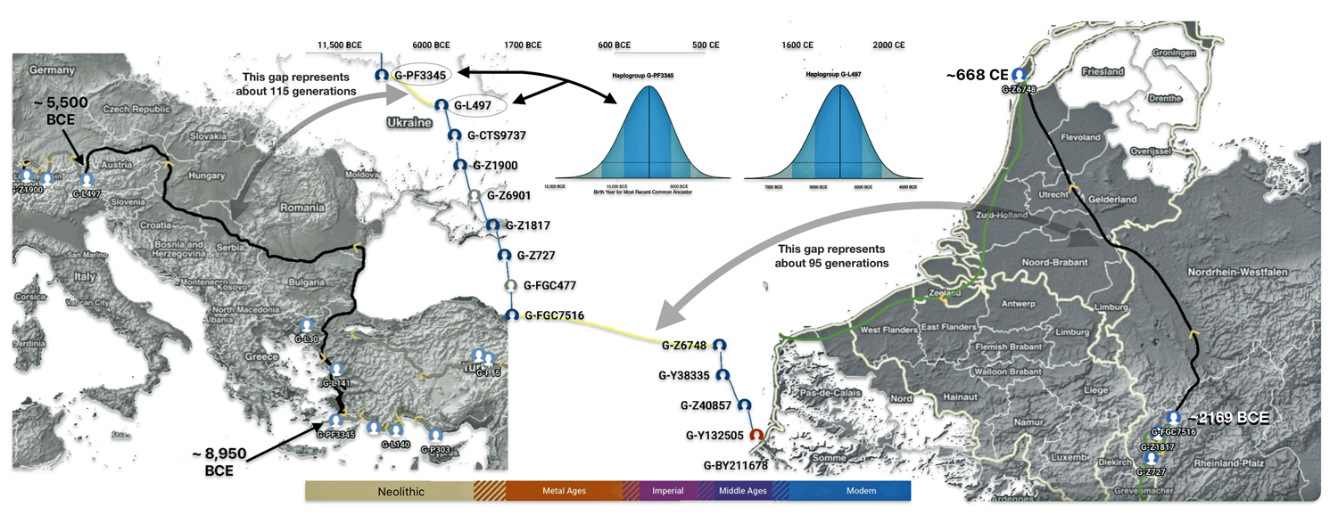
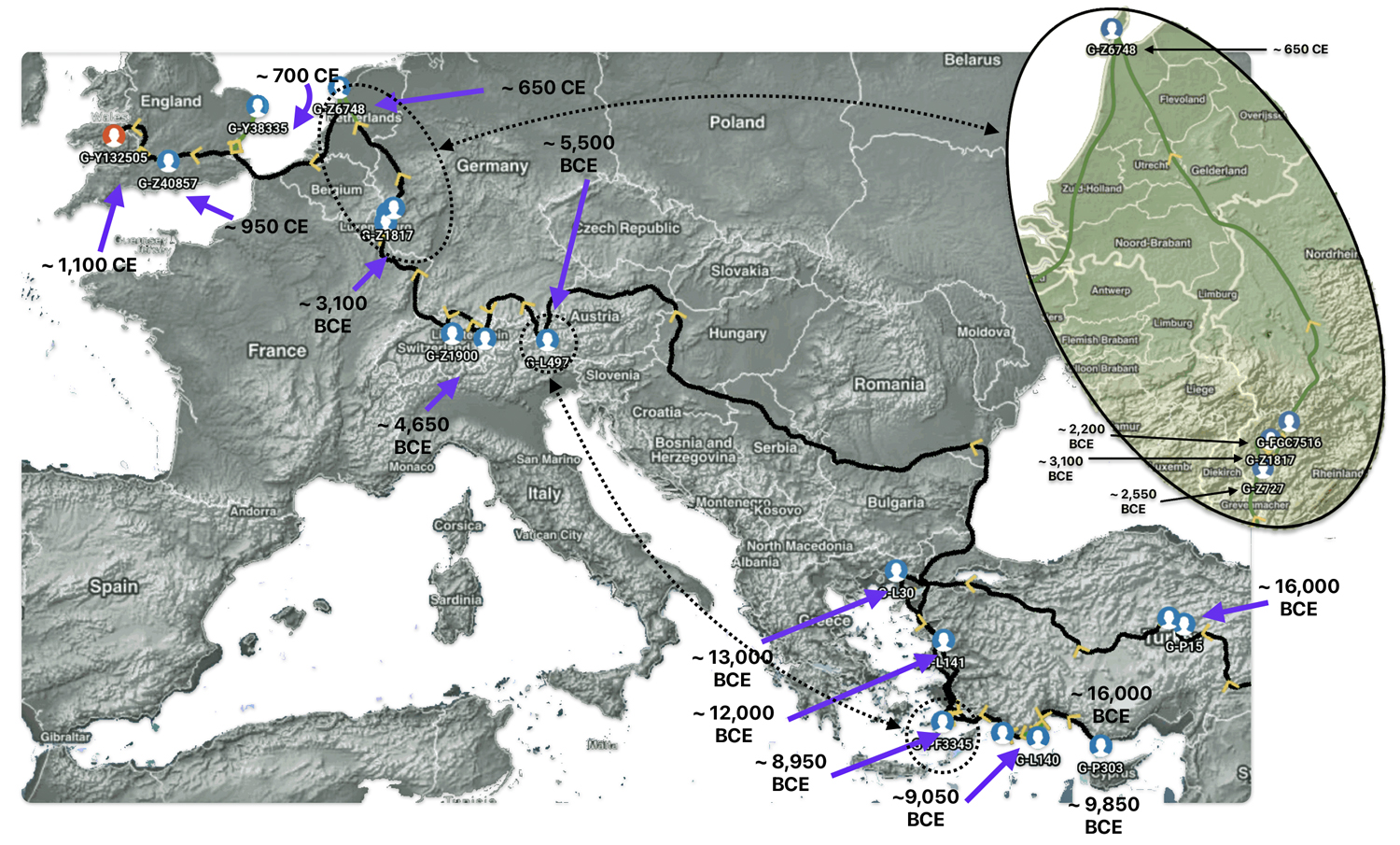
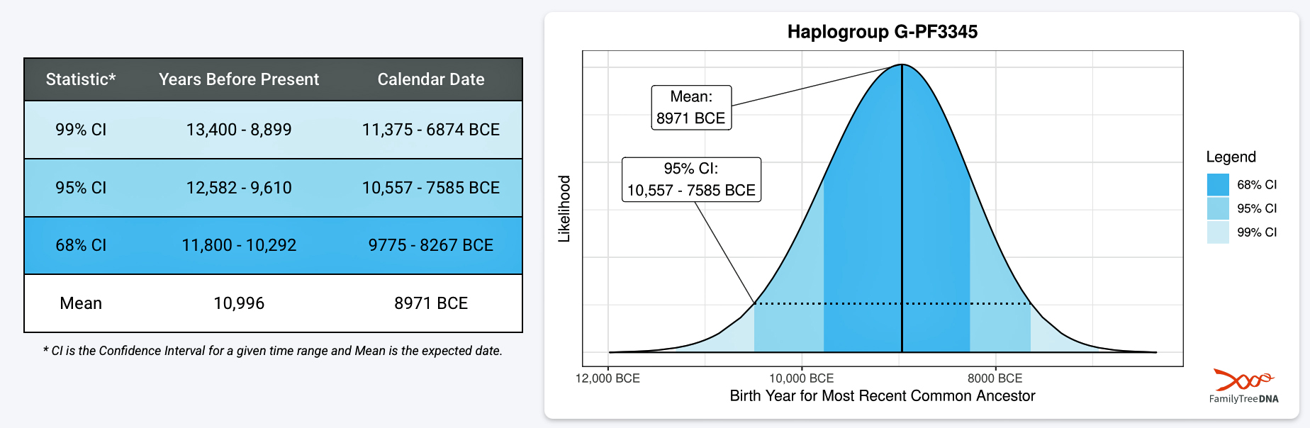
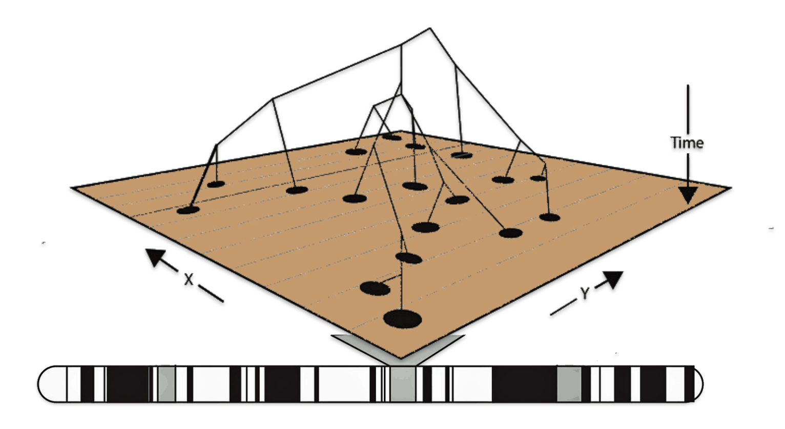
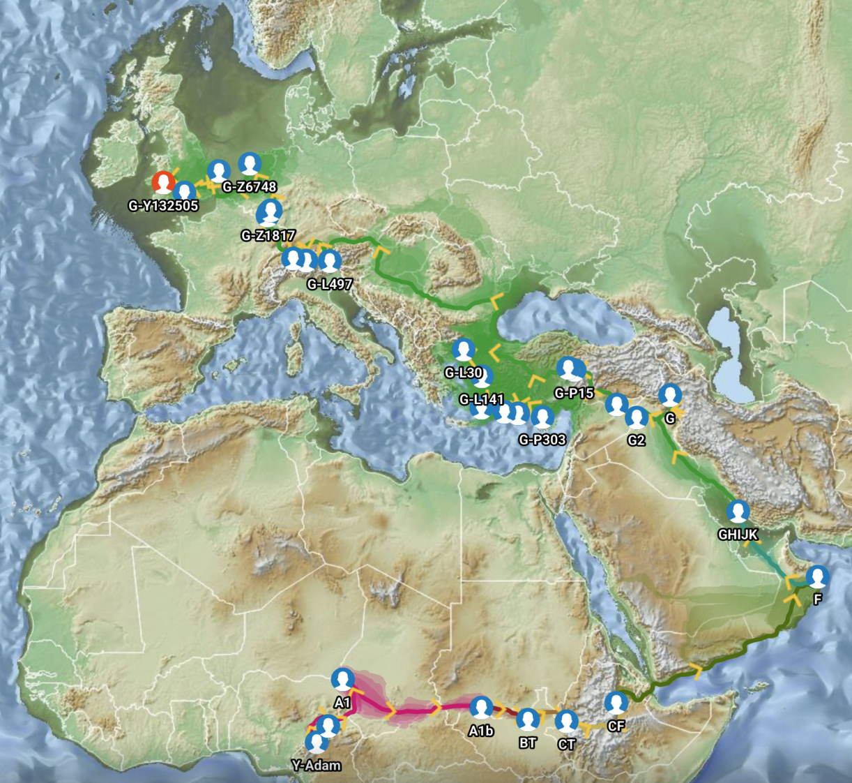
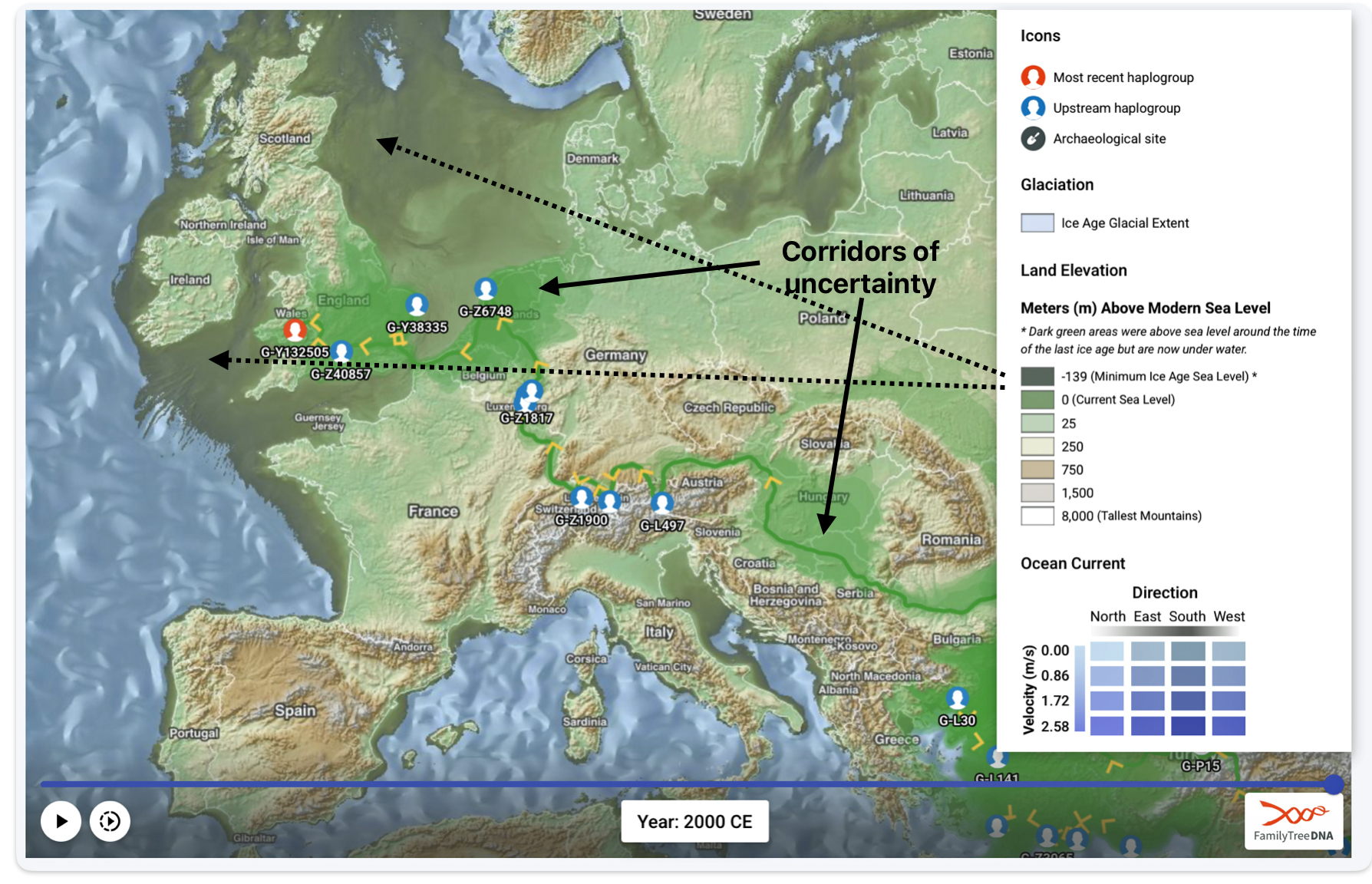
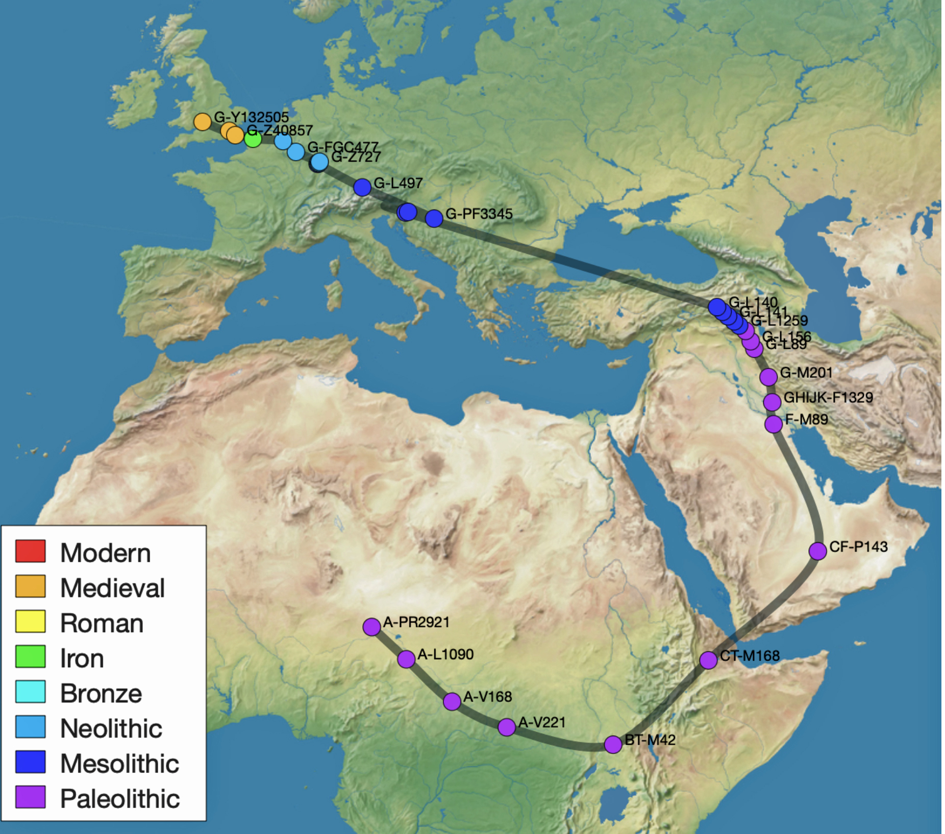
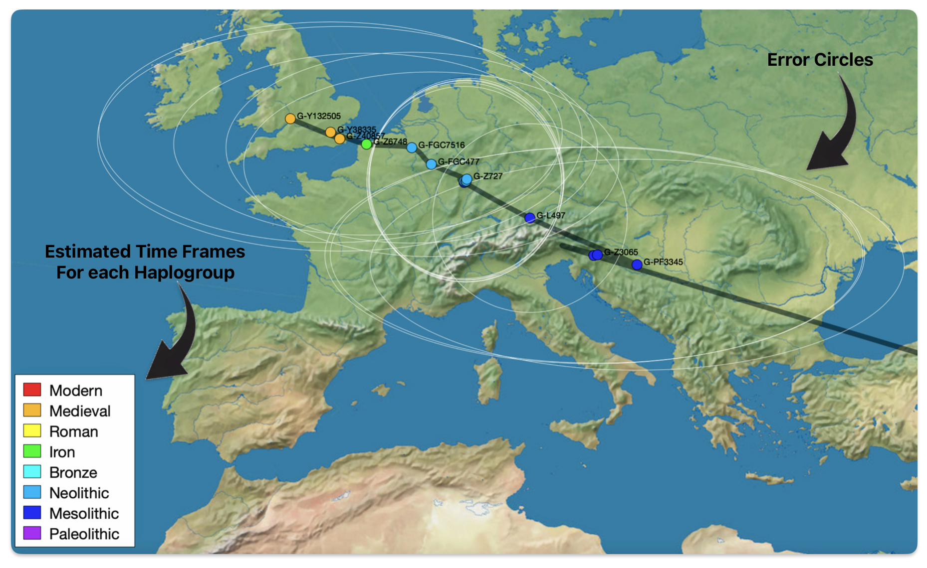
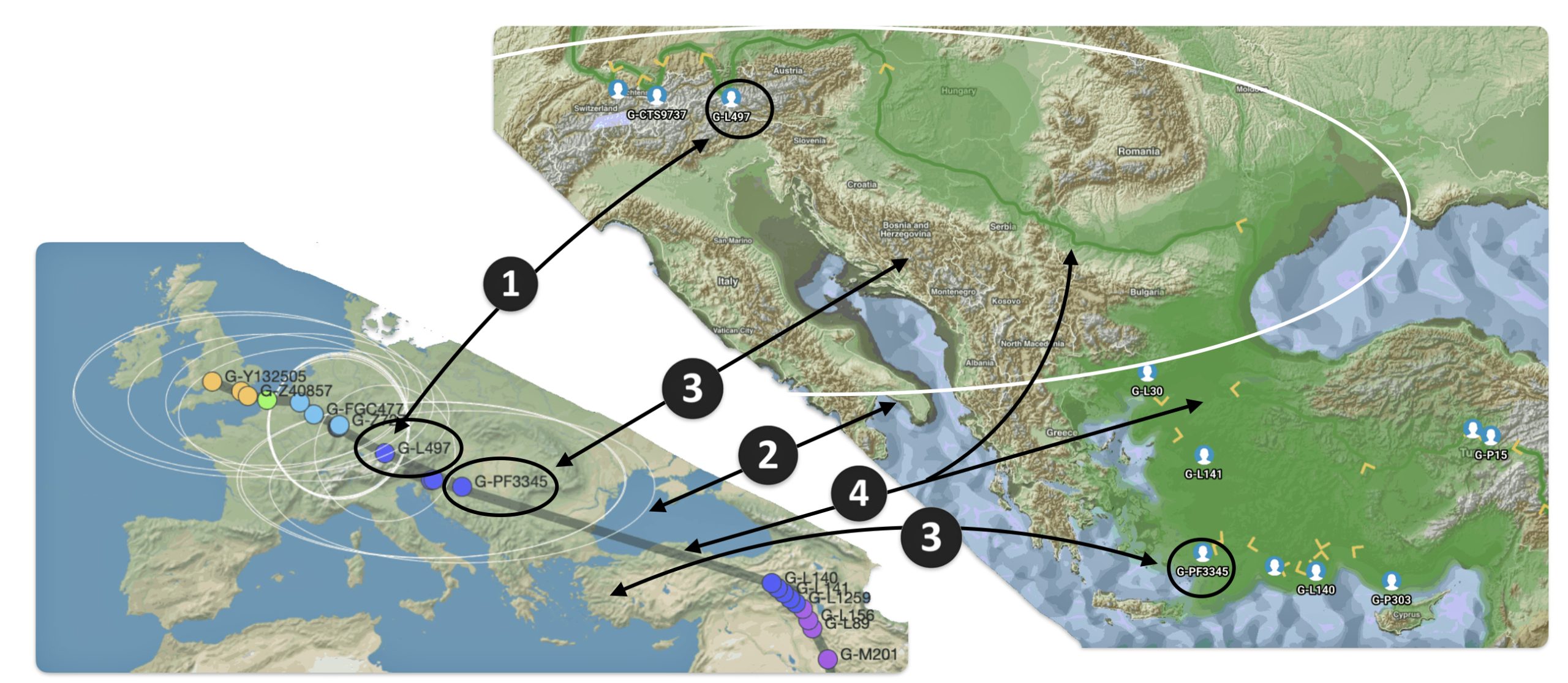
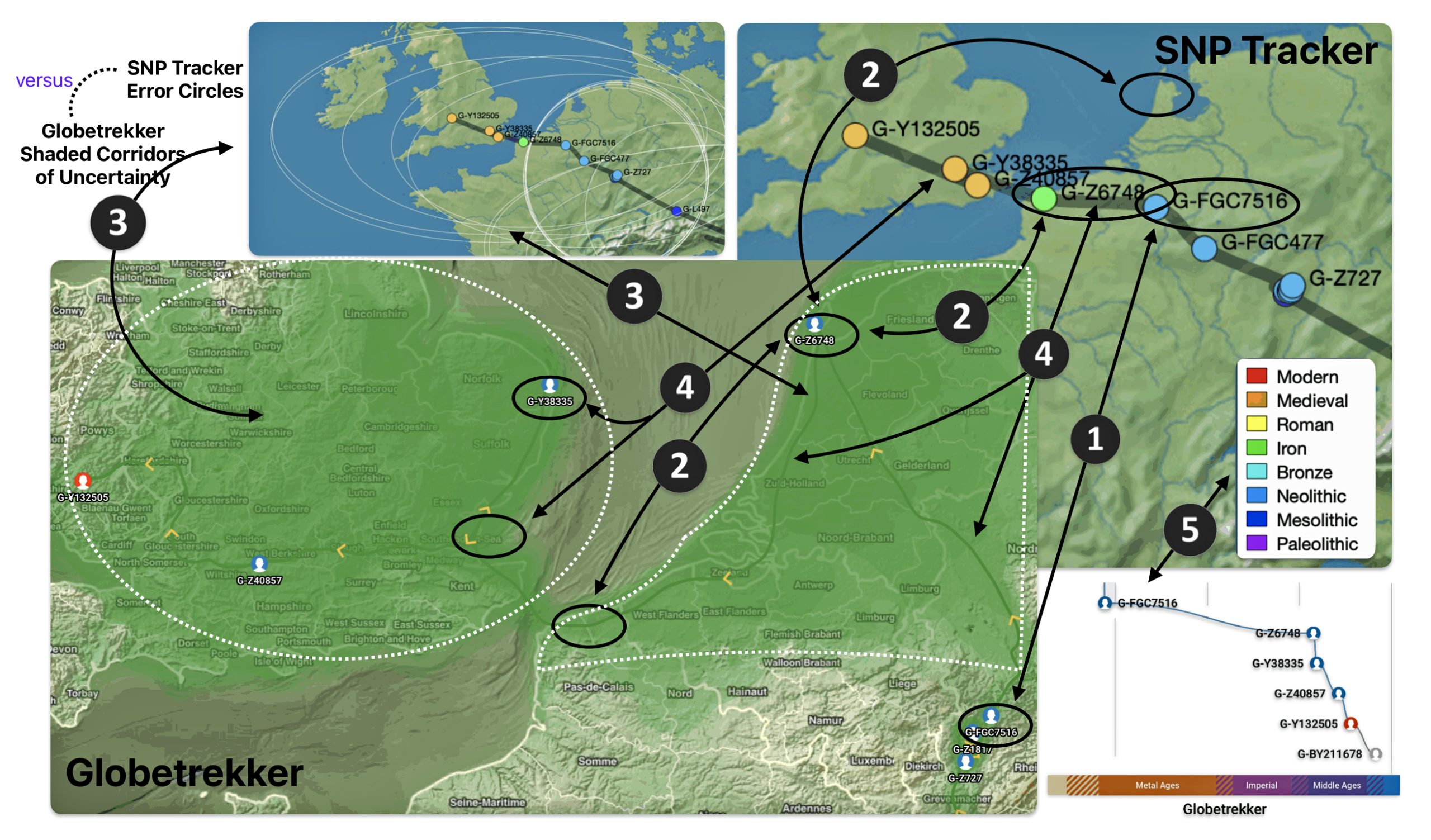