
Genealogical time takes on different meanings and reality depending on which methods are utilized to analyze evidence. Our terminology consequently changes and the focus of our story changes as we go back in time. We gradually start looking at our respective family descendants not in terms of their family roles as father, uncle, and great grand mother but in terms of genetic mutations.
The concept of generations morphs into genetic distance. [1] Our focus on the family tree branches and families shifts to the analysis of genetic lineages and haplogroups. [2] Our individually identified descendants such as a great4 grandfather or our great4 grandmother are shifted to identifying the Most Recent Common Ancestors (tMRCA). [3]
Genealogical time shifts our focus on ethnic backgrounds and origins obtained from autosomal DNA tests to analyzing migratory patterns of haplogroups and determining the presence of ancient cultures that might correlate with where our genetic descendants may have lived. The analysis of Y-DNA or mtDNA extends genetic links backward in time thousands of years. The notion of ‘ethnic origin or composition’ becomes less important since ethnicity is largely the product of cultural patterns dependent upon historic time and location.
“As a scientist, I find questions of identity and ethnicity to be simplistic and naïve. The answer depends on “which branch?” and “when?”. In my case, if when = now, I’d say a retiree from Connecticut. If when = 1800 on my paternal line, I’d say a farmer from Vermont. If when = 1600, then a sheep herder in Bedfordshire England. In the Roman era, probably north central Europe; in Mesolithic era, in the Balkans. And if when = 35,000 years ago or before, then my ancestors were African hunter-gatherers, like all of us.” [4]
Genetic genealogy introduces a different view of time and the analysis of ‘genealogical facts’ through different layers of time. The notion of time radically expands in scope and changes how we perceive and measure change and time and view genealogical evidence.
This story presents a view that the different approaches and related methodologies for conducting genealogical research depict three different interrelated historical layers of time. While each historical layer has distinctive properties, the boundaries between each are not clearly defined and can shift on the basis of genealogical discoveries. Each layer has different rhythms of time. Each historical layer has different conceptions of reality as perceived by the genealogist and also exhibits different properties of reality.
Among the many influences on my views on genealogical layers of time, there are three individuals that are notable. Two of the three are genetic genealogists J.David Vance and Rob Spencer. The third influence is an historian Fernand Braudel, who was an historian from the Annales School of French historiography and social history. [5] In addition to traditional notions of history, Braudel introduced the concepts of longue durée and conjunctures to analyze historical cycles. [6]
Vance’s View of Genealogy as Having Three Historical Phases
J. David Vance is a prominent genetic genealogist with over 35 years of traditional genealogy experience and has been actively involved in genetic genealogy projects and organizations since 2005. At the time of writing this post, he served as the Senior Vice President and General Manager at FamilyTreeDNA.
Vance advocates for a more inclusive approach to family research that combines traditional genealogical methods with genetic testing, acknowledging both biological and non-biological family connections. His work particularly emphasizes helping traditional genealogists transition to incorporating DNA evidence in their research, while maintaining a balanced perspective that values both documentary and genetic evidence in family history research. [7]
Vance’s Continuum of Genealogical Time Through Y-DNA Testing
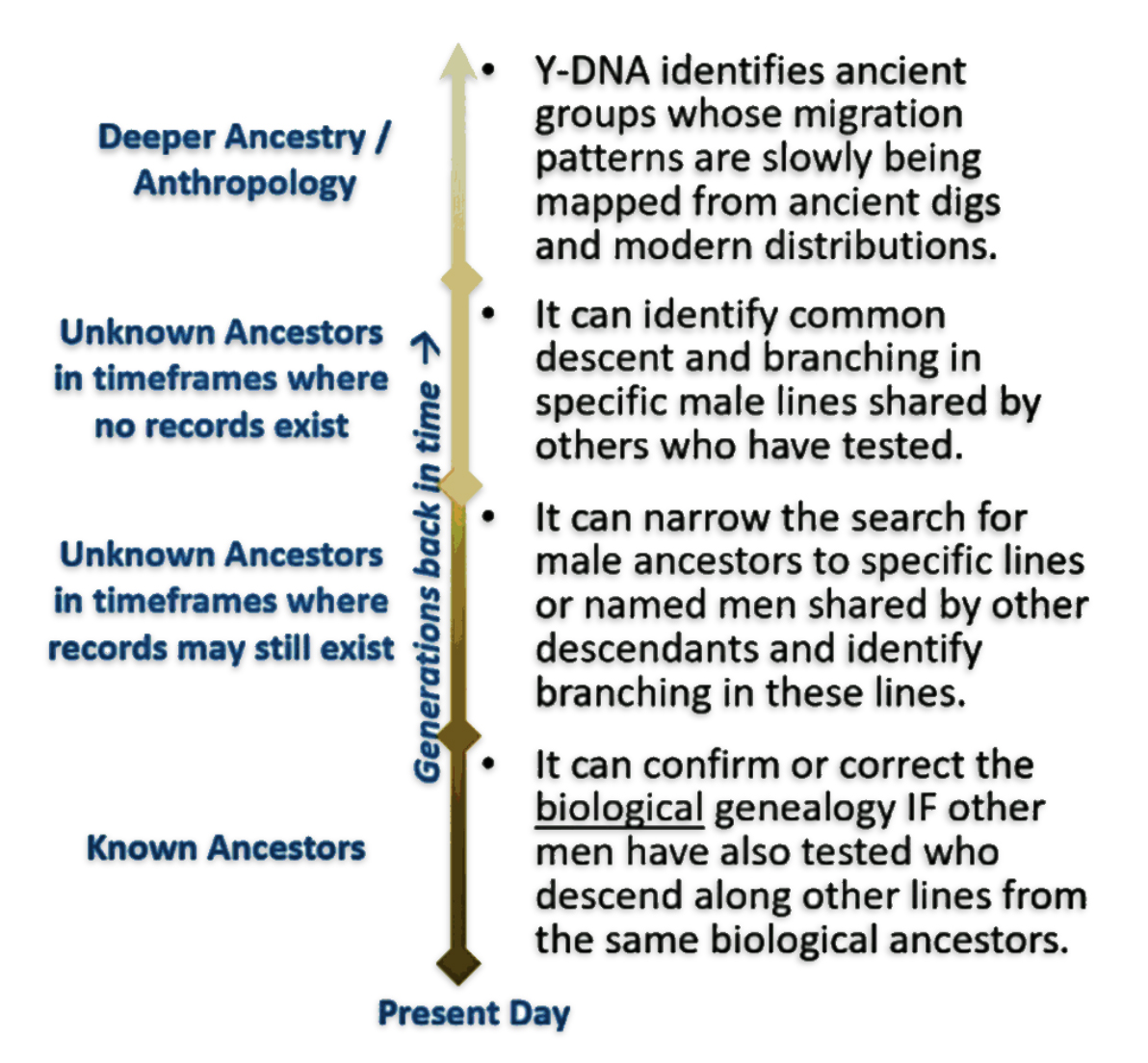
Vance is known for developing innovative approaches and technical contributions [8] to understanding genetic genealogy, including his metaphor comparing traditional genealogy to building a mansion with portraits, and genetic genealogy to adding stained-glass windows with DNA patterns. [9] His ‘three phases of genealogy’ has had a major impact on my thinking about the relationship between traditional and genetic genealogy and the strategy of using both in genealogical research.. [10]
Illustration One: The Three Phases of Genealogy
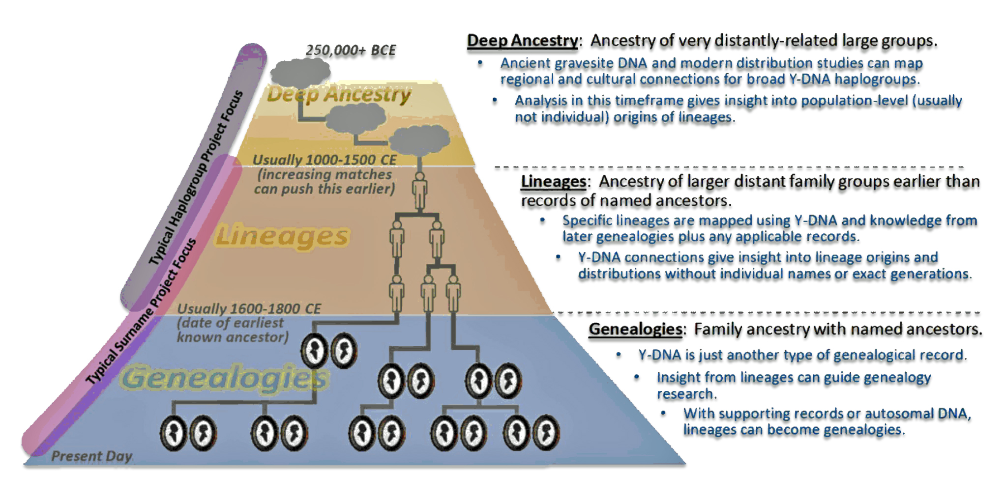
David Vance uses the term ‘genealogy‘ to demarcate a period of time where generations of named ancestors have been documented through traditional records research and possible DNA testing. DNA tests are just another source or corroborating type of genealogical record.
Beyond this period is a time which is beyond many of our “brick walls” of genealogy. This is where we cannot trace our family tree further into the past. Vance calls this netherworld time period as the period of lineages. The line of demarkation between lineages and genealogy is not hard fast period of time and it can change based on genealogical discoveries.
“. . . (I)n between deep ancestry and the genealogy of named ancestors (traditional genealogy), we have what (are) “lineages” for lack of a better term. These are genealogies if you will but of unnamed ancestors over a period of time when you have known (genetic) interconnections.
“The generations may be estimated, the timeframes may be estimated, but you know that the connections happened because the Y-DNA tells you that there were mutations that were passed on by men who lived in those time periods and those men had descendants who had further mutations and so you can map the family relationships between those men even if you can’t ever name them. ” [11]
This period is still within historical times where one can amass enough DNA information about the timeframe in which the DNA matches lived to possibly develop strong working hypotheses about unnamed ancestors. It is possible to isolate the region where several generations of unnamed ancestors lived, what possible surnames they had, or identify what emerging country or ethnic group that may have been part of in that particular geographical area.
“Lineages are a way that Y-DNA (or mtDNA) can extend our knowledge of our ancestry beyond we would have thought possible in ‘regular’ genealogy – we can learn about our ancestry even before the time of records. We can map the branching points between ours and our matches’ lines and understand the order and approximate time frame in which our common ancestors lived. We can collect the known information about all the descendant lines from these ‘lineage ancestors’ and draw conclusions about where and perhaps how they lived.” [12]
At some point in time the period of lineages end. However, genetic genealogical testing and research can help bridge the gap to go even further back in time. The period beyond lineages is what Vance calls ‘deep ancestry‘. Deep ancestry is characterized by the mapping of haplogroups based on genetic mutations. These are various haplogroups of descendants that are connected by a common Y-DNA or mtDNA mutation that occurred in a common ancestor, the most recent common ancestor (tMRCA). These mutations can be mapped out in what is known as a haplotree. [13] While Haplogroups can be defined during the time of lineages and genealogies, in the era of deep ancestry it is the only information that might be available for one’s ancestral lineage.
Spencer’s View of Three Different Research Levels
The other genealogist that has influenced my view of geological time is Rob Spencer. Spencer specializes in analyzing genealogical genetic and historic data at the macroscopic level. His main interests are the exploration of genetic genealogy and population genetics at the macro level. His work specifically focuses on analyzing ‘monoparental’ SNPs (mutations in Y and mitochondrial DNA) to trace ancestral migration patterns from prehistoric times to the present. His emphasis is getting the most out of Y-DNA data by applying original algorithms to create informative graphics. [14]
Spencer’s talent and expertise is reflected in the creation of online mathematical modeling tools to analyze large samples of genetic test results and historical data. (See illustration two.) He provides innovative ways to analyze data and graphically portray results in intuitive and elegant ways. He actively shares his knowledge and mathematical applications through presentations and online documentation. [15]
Illustration Two: Spencer’s Online Tools and Data Sources
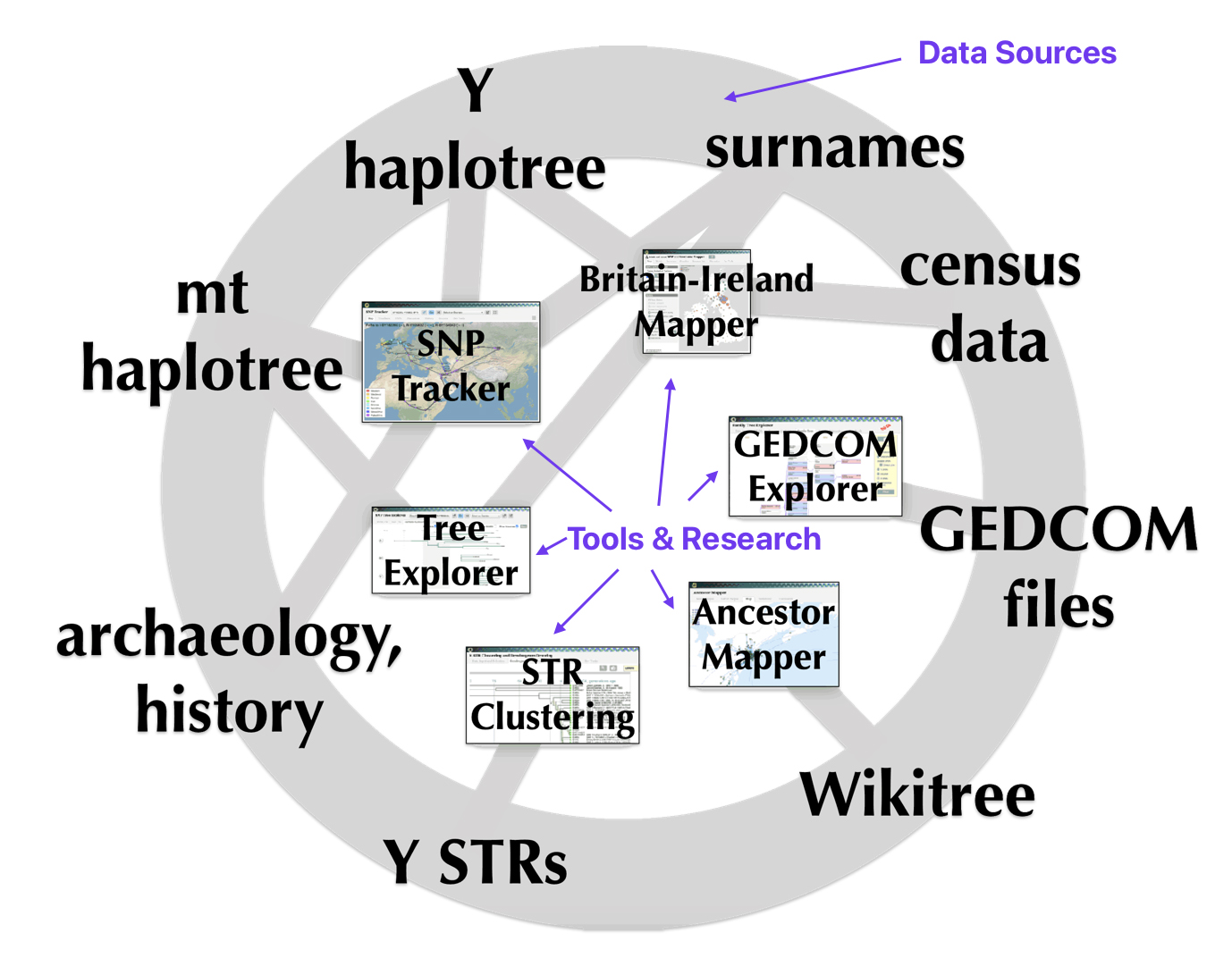
I have utilized many of Spencer’s online mathematical tools to analyze Y-STR and Y-SNP test results and his map modeling of surname distributions in Wales. Two of his more popular online programs are the SNP Tracker, a tool that helps genealogists track and map the migration paths of Y-SNP genetic mutations through time, and the Y STR Clustering and Dendrogram Generation tool, which provides a graphic portrayal of the genetic distance of between Y-DNA testers.
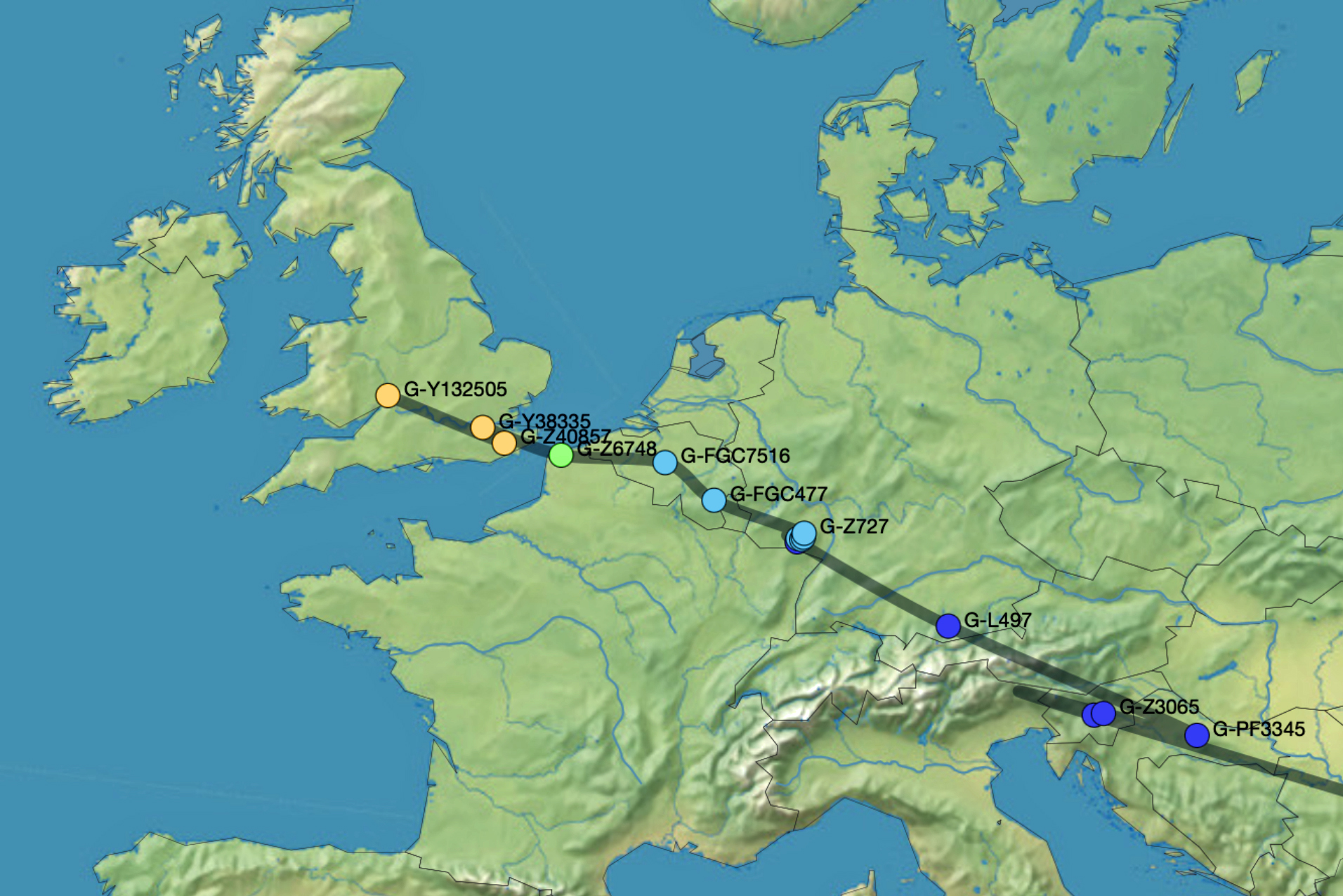
The SNP tracker is particularly useful when tracking Y-DNA SNP lineages in Vance’s Deep Ancestry phase and the Period of Lineages. Illustration three depicts the general mogratory path of my Y-DNA linneage in the past 10,000 years.
Illustration Three: Example of Results of Spencer’s SNP Tracker Using My Lineage of SNP Mutations from my DNA Test Results
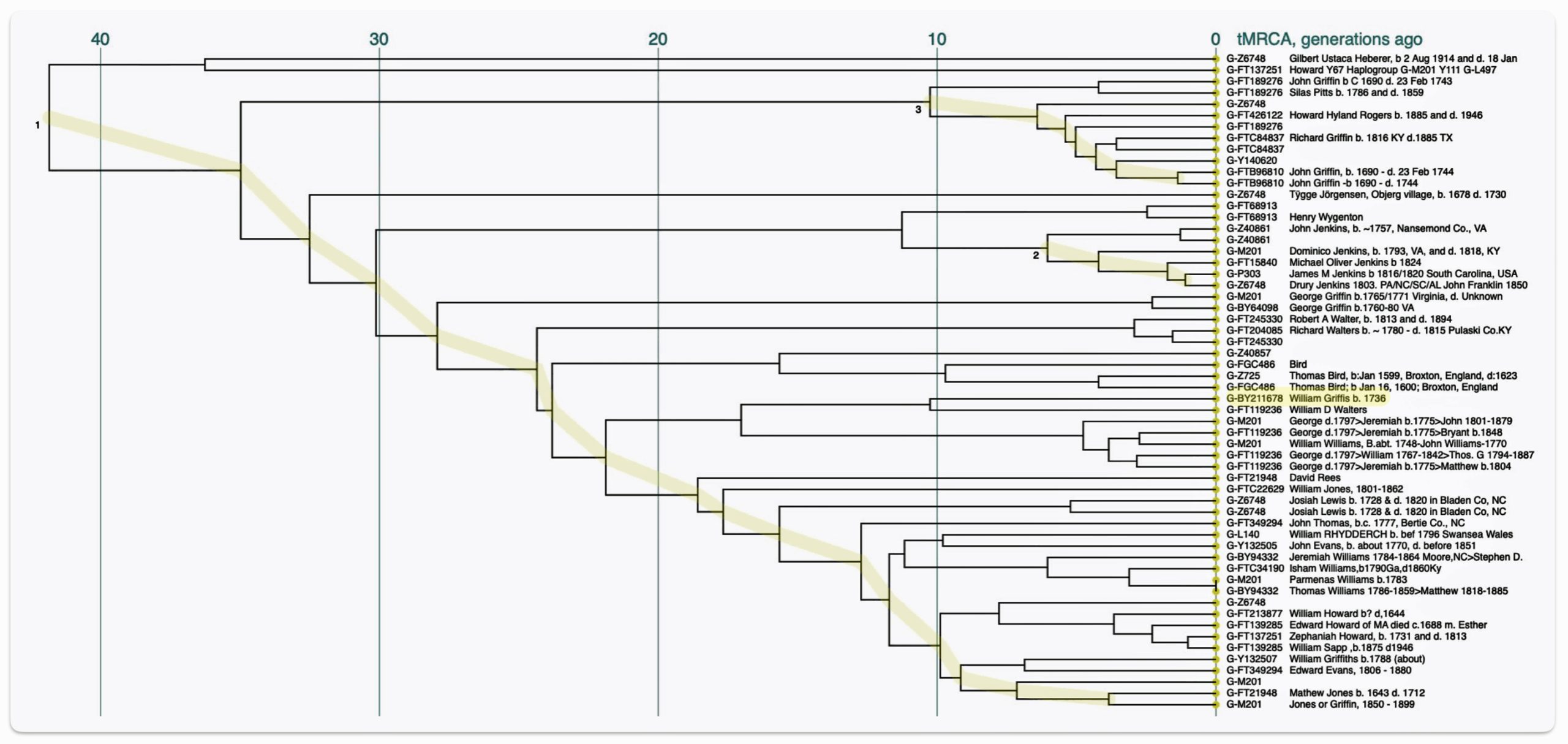
The STR Clustering and Dendrogram Generation Tool is very useful in visualizing genetic distance between Y-DNA testers in the context Vance’s Period of Lineages and the Period of Traditional Genealogy. (See iIllustration four.) [16]
Illustration Four: Example of Using Spencer’s STR Clustering and Dendrogram Generation Tool with FTDNA Y-DNA Test Kit Results that are part of the G-Z648 Haplogroup Branch
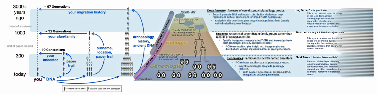
Similar to David Vance’s three periods of ancestry, Rob Spencer provides a graphic portrayal of tracing one’s ancestor’s based on three levels of research (illustration five).
Traditional genealogical paper trails and research can provide information in the recent past. Beyond 300 years, the paper trail tends to thin out and evaporate. In this research level, genetic genealogy is often used to confirm or refute traditional paper evidence. [17]
Ancestry between 300 and about 1000 years ago depicts a period where surnames may exist but paper trails are not available. For certain European areas on the British Isles, extended Y-DNA genetic lineages with different surnames can be located fairly accurately by date.
Illustration Five: Three Levels of Genealogical Research

The research strategy for genetic genealogy beyond 1,000 years can utilize Y SNP DNA to document genetic lineages through SNP mutations and can be expressed as a haplotree, essentially a family tree that branches at SNP mutations.
“A variety of methods (ancient skeletal DNA, modern tester citations, surnames and census data, and mathematical modeling) can be used to locate SNP events in space and time across the globe, after which simply knowing one’s most recent SNP suffices to reveal a personal paternal journey. Several examples illustrate the great diversity of our paths and origins. The Y haplotree is now so detailed that the SNP trail frequently overlaps paper genealogic records, providing a complete path from paleolithic Africa to the modern era.” [18]
Spencer has documented the utility of analyzing Y STR genetic pair-wise data test results to tease out the genealogical evidence between what he calls your ancestry, your clan, and your migration history levels of research. The illustration provides a good graphic relationship between traditional and DNA based genealogical research.
The use of Y-DNA research can help trace unknown ancestors prior to the use of surnames, pinpoint possible regional areas where ancestors lived, and provide possible links to the recent past. Y-DNA research, coupled with archaeological and paleo-genomic discoveries can also shed light on macro level connections to migration patterns that can be associated with genetic ancestors. [19]
Braudel’s three periods of historical time
As indicated in a previous story, social historians and micro-historians have influenced my approach in developing stories of ancestors. All of these stories involve family subject matter that occurred within the last 10 generations or roughly 300 years ago.
The writings of French historian Fernand Braudel have influenced my way of thinking in another way. Braudel’s work underscores the importance of long-term rhythms and multiple temporal cycles and scales in understanding human history and placing genealogical analysis in this broader view. Ferdinand Braudel’s all encompassing historical method has provided a conceptual historical framework akin to the quest for a unified theory of physics. He has been referred to as “ a grand panjandrum—slightly emeritus—of history.” [20]
Notwithstanding his critics, [21] Fernand Braudel was an extraordinary figure in the field of history. His extensive historical research, unique approach, and innovative concepts have left a lasting impact on the way civilizations as well as everyday people in specific time periods can be understood. His work also highlights the role of geography and time in shaping human agency. Braudel revolutionized historical analysis by introducing a three-tiered approach to understanding historical time, moving away from traditional history focused on political events and “great men”. [22]
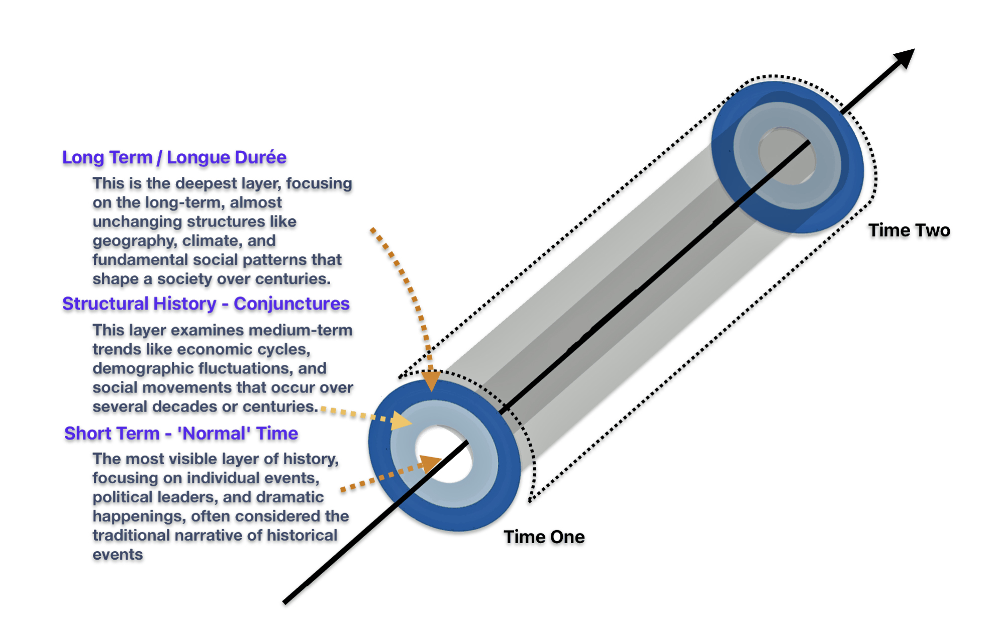
Braudel rejected simple chronological time in favor of three interrelated layers of historical duration: [23]
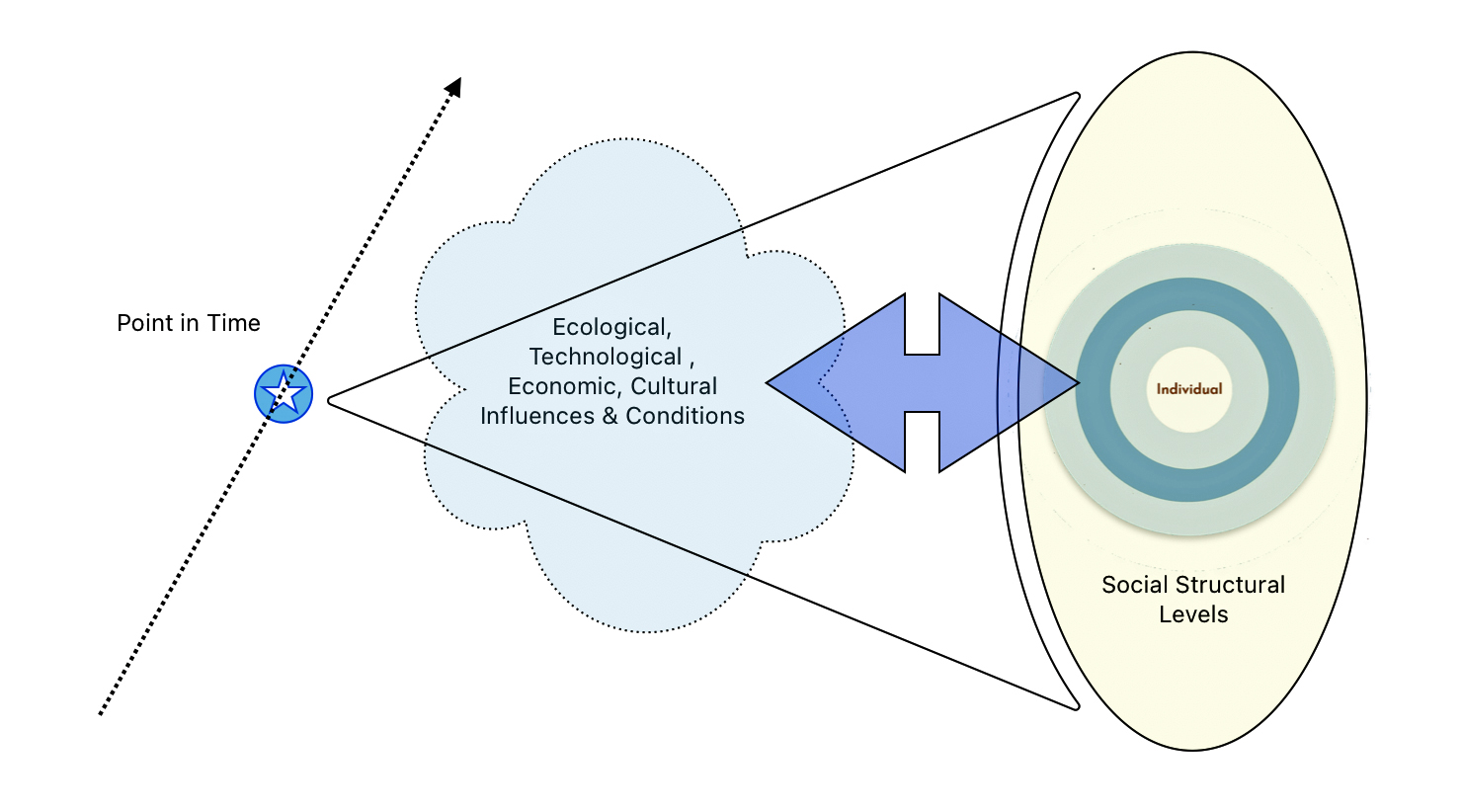
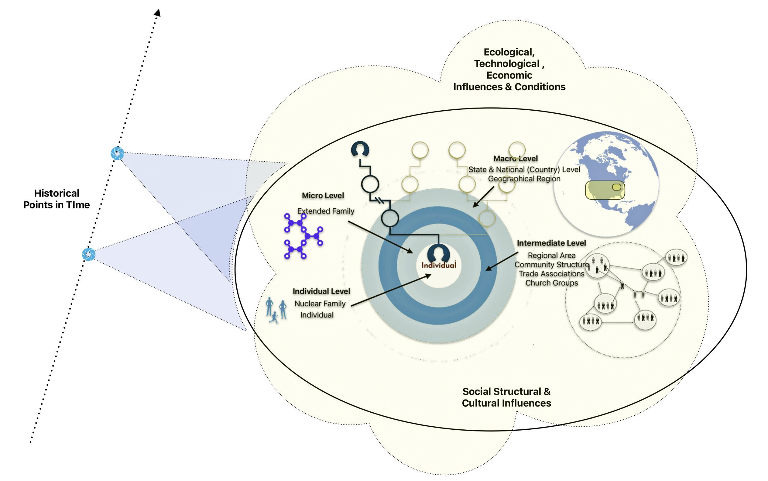
- The longue durée focused on slow-moving geographical, environmental, and structural patterns. The slowest and most fundamental level involves environmental and geographical changes, characterized by slow, almost imperceptible shifts and recurring cycles. This forms the backdrop against which all human activity takes place, including the relationship between people and their environment.
- Medium-term conjunctures covers economic cycles and social trends. The intermediate level encompasses long-term social, economic, and cultural patterns, typically spanning from a number of generations to two to three centuries. This includes phenomena like economic cycles, demographic shifts, changes in state level dimensions, and Industrial and agrarian growth patterns.
- Short-term events (histoire événementielle) deals with surface-level political events and individuals. The most immediate level deals with individual actions, political events, and ‘surface-level’ occurrences. Braudel considered this the least significant level for understanding deeper historical processes.
Illustration Six: A Depiction of Braudel’s Three Layers of Time
Braudel broke from traditional narrative history by rejecting the focus on political elites and “great men” in favor of examining marginal people like slaves, serfs, and the urban poor. He also believed in integrating multiple social sciences into historical analysis. His historical analysis emphasized objective forces over individual human agency in shaping history. For Braudel, the subject matter of history is influenced based on the scale of time that is used to analyze the past. The rise and fall of states, and the short-lived and dramatic moments of the lives of “great men” are replaced by the long-term rhythms of material life.
Braudel’s examination of material life between 1400-1800 in Europe demonstrated how daily life and progress were shaped by these temporal rhythms. His approach combined multiple disciplines, particularly geography and economics, to create a comprehensive view of historical development. [24]
His historical work is impressive with great detail on the wide range of material elements of daily life that influence the how history unfolds at the the individual level and throughout various social levels (local, national, regional , etc). This method allowed him to demonstrate how trading routes, sailing patterns, and economic structures influenced societies over extended periods.
His innovative perspective transformed historical study from focusing solely on political events and “great men” to examining the deeper, more persistent patterns of human civilization. This approach particularly emphasized how material conditions and environmental factors created enduring structures that shaped human possibilities and constraints over centuries. [25]
Braudel also demonstrated quite clearly that history does not exist independently of the historian’s perspectives and prejudices. As with specialists in other disciplines, the historian intervenes at every stage in the making of history.
“All historical work is concerned with breaking down time past, choosing among its chronological realities according to more or less conscious preferences and exclusions. Traditional history. with its concern for the short time span, for the individual and the event, has long accustomed us to the headlong, dramatic. breathless rush of its narrative.
“The new economic and social history puts cyclical movements in the forefront of its research and is committed to the time span. … side by side with traditional narrative history, there is an account of conjunctures which lay open large sections of the past, ten, twenty, fifty years at a stretch ready for … examination.
“Far beyond this second account we find a history capable of traversing even greater distances. a history to be measured in centuries … the longue durée. ” [26]
There is a long litany of scholarly articles and debates on Braudel’s work and the utility of what are the various periods of historical time. I wish to deflect the path of discussion to what his work inspires when it comes to doing genealogical research. I might be oversimplifying or misconstruing his model of historical method so I beg forgiveness in advance. Nevertheless, I share the opinion that the three temporalities of genealogy and history is a useful methodological framework to guide research.
“The longue durée is simply the most stable temporal relation of the longest duration in the problem under consideration. It forms the stabilizing ground against which cyclical variations of other temporal structures are established, and it allows the ordering of historical inquiry.
“It is, in the final analysis, a methodological tool that is constructed for the analysis of particular problems. It is based on a particular focus of one’s research and not necessarily an objective time period that stand alone.” [27]
The ‘longue durée or the long duration for Braudel forms the stabilizing ground against which cyclical variations of other temporal structures or influences are established. It allows the ordering of historical inquiry.
“It is simply the most stable temporal relation of the longest duration in the problem under consideration. It forms the stabilizing ground against which cyclical variations of other temporal structures are established, and it allows the ordering of historical inquiry.” [28]
A Model of Genealogical Time
On the surface, there are strong similarities between the three layer concept of genealogy between Vance and Spencers’ perspectives. Each of their respective genealogical layers or stages of genealogy and research involve similar boundaries of time between traditional genealogy, the period of lineages or clans, and deep ancestry or migration history. References to the Longue Durée have been alluded to in genetic studies. [29]
Braudel’s three temporal layers can provide a comprehensive framework for integrating traditional and genetic genealogical research. The Longue Durée, the foundational layer, can provide an understanding of the correlation between haplogrop migration and the geographical location with:
- ancient cultural groups that existed in specific geographical areas;
- long-term climate and landscape changes that affected areas where haplogroups lived and migrated; and
- geographic patterns of DNA distribution across regions that shaped ancestral migrations. [30]
Braudel’s middle or conjuncture layer of time reveals long historical cycles that can be correlated with historical events in time. This middle layer of time can also be viewed within a genetic genealogical perspective that focuses on Y-STR mutations within Vance’s period of lineages or Spencer’s period of clans. The middle historical time layer can be viewed in terms of tracing SNP and STR Y-DNA mutations in lineages and haplogroups. This historical time layer focuses on:
- demographic shifts and genetic lineage patterns across multiple generations;
- economic cycles and other social structural patterns that can be identified with migration patterns and movement of lineages and haplgroups;
- cultural groups that can be correlated with the location of lineages and clan groupings; and
- the identification of surname formation among lineage groups.
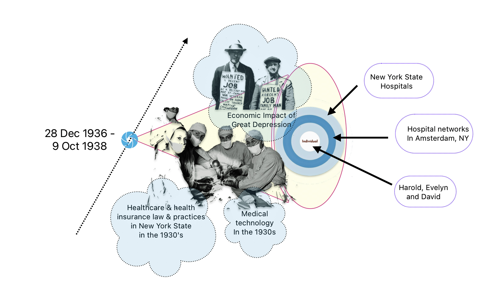
Braudel’s ‘event’ layer aligns with traditional genealogical research. Historical events can be identified with family historical stories in the context of the four structural levels identified in a prior story. DNA matches showing recent common ancestors in the last 10 generations can also be aligned with traditional genealogical research. .
By combining these layers, genealogists can contextualize genealogical evidence within broader social and environmental patterns; use genetic data to confirm documentary evidence; and connect individual family events to larger historical forces that shaped ancestral patterns. [31]
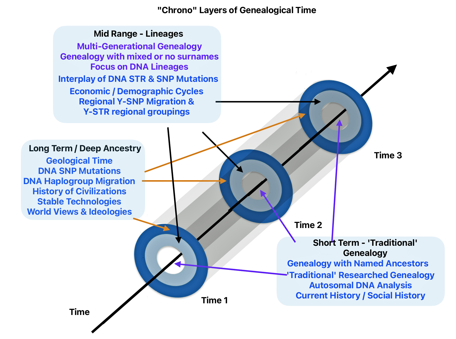
This multi-layered approach to genealogical time helps overcome research barriers by providing alternative perspectives when one type of evidence is lacking. The resultant model based on the three major influences discussed above is reflected in illustration seven.
Illustration Seven: Chronological Influences on Genealogical Research
Continuation of the Story
The second part of this story on genealogical time discusses how family history stories that incorporate the three layers of genealogical time will draw on different sources of evidence. The orientation of the narrative of a story will be uniquely tailored based on the sources of evidence..
Sources
Feature Image: The image is a collage of illustrations of genealogical and historical time based on models provided by J. David Vance, Rob Spencer and Fernand Braudel.
[1] Genetic distance measures the number of differences or mutations between two individuals’ DNA test results.
For Y-DNA analysis, a genetic distance of zero indicates an exact match between two people’s DNA results, while higher numbers indicate more genetic differences. It counts the number of mutations between two men’s Y-chromosome DNA results. Each genetic marker difference contributes to the total genetic distance. For example, if one person has a value of 10 at DYS454 and another has 11, this contributes a genetic distance of 1. DYS stands for DNA Y-chromosome Segment in genetic research. It refers to a short tandem repeat (STR) found on the Y chromosome.
For autosomal DNA research, genetic distance measures the length of shared DNA segments in centiMorgans. It is used to determine relationships between any two people, regardless of gender.
Genetic distance is not a direct measure of generations between individuals, but rather indicates genetic divergence. A smaller genetic distance suggests: closer genetic relationship between individuals, a more recent common ancestor, and an higher likelihood of genealogical connection.
The interpretation of genetic distance values varies depending on the number of markers tested in Y-DNA tests, with different significance levels for 37-marker, 111-marker, and Big Y (700 marker) tests.
Genetic Distance, International Society of Genetic Genealogists Wiki, This page was last edited on 31 January 2017, https://isogg.org/wiki/Genetic_distance
Estes, Roberta, Concepts – Genetic Distance, 29 Jun 2016, DNAeXplained – Genetic Genealogy, https://dna-explained.com/2016/06/29/concepts-genetic-distance/
Genetic Distance, Wikipedia, This page was last edited 25 Oct 2024, https://en.wikipedia.org/wiki/Genetic_distance
Understanding Y-DNA Genetic Distance, FamilyTreeDNA Help Center, https://help.familytreedna.com/hc/en-us/articles/6019925167631-Understanding-Y-DNA-Genetic-Distance
Mohler, Melanie, Genetic Distance | YDNA Matches, 3 Jan 2023, Your DNA Guide, https://www.yourdnaguide.com/ydgblog/genetic-distance
[2] A genetic lineage encompasses all descendants of a specific genetic sequence that typically emerges after a new mutation. This concept differs from an allele as it includes descendants with additional mutations while excluding cases where different mutations create the same allele. An allele is a variant form of a DNA sequence at a specific location (locus) on a chromosome. Humans inherit two alleles for each gene. Alleles can differ through single nucleotide polymorphisms (SNPs) or have insertions and deletions of thousands of base pairs. While most allelic variations cause little change in gene function, some can result in different observable traits.
A haplogroup is a genetic population group of people who share a common ancestor and specific genetic mutations. These groups are defined by shared inherited genetic markers that are passed down through either the paternal line (Y-DNA) or maternal line (mitochondrial DNA).
Lineage (genetic), Wikipedia, This page was last edited on 28 August 2024, https://en.wikipedia.org/wiki/Lineage_(genetic)
Haplogroups are identified by initial letters of the alphabet, with refinements using additional number and letter combinations (e.g., A → A1 → A1a). They form a nested hierarchy, where each haplogroup remains part of a preceding haplogroup.
Haplogroups help trace human migration patterns and evolutionary history, connecting modern populations to their ancient ancestors. They originated in Africa and diversified as humans migrated across continents, developing new mutations that created distinct regional patterns.
Haplogroup, Wikipedia, This page was last edited on 8 December 2024, https://en.wikipedia.org/wiki/Haplogroup
Haplgroup, International Society of Genetic Genealogy Wiki, This page was last edited on 1 November 2024, https://isogg.org/wiki/Haplogroup
Estes, Roberta, What is a Haplogroup?, DNAeXplained – Genetic Genealogy, https://dna-explained.com/2013/01/24/what-is-a-haplogroup/
[3] In genealogy research, the “most recent common ancestor” (MRCA) refers to the most recent individual from whom two or more people are directly descended, essentially the point in a family tree where two lineages converge and share a common ancestor; it is the closest ancestor that two individuals share based on their genetic lineage.
Most recent common ancestor, International Society of Genetic Genealogy Wiki, This page was last edited on 31 January 2017, https://isogg.org/wiki/Most_recent_common_ancestor
Most Recent Common Ancestor, Wikipedia, This page was last edited on 5 November 2024, https://en.wikipedia.org/wiki/Most_recent_common_ancestor
[4] Spencer, Rob, Welcome , Footnote on home pageTracking Back, https://scaledinnovation.com/gg/gg.html?nm=welcome
[5] The Annales School is a French historical movement founded in the early 20th century that revolutionized historical research by emphasizing long-term social history over traditional political and military narratives. Marc Bloch and Lucien Febvre established the movement in 1929 by founding the journal “Annales d’histoire economique et sociale”. The Annales School transformed historical research by expanding its scope beyond traditional political narratives to include the study of ordinary people, social structures, and long-term historical patterns.
The school developed several innovative approaches to historical study. The Annales School emphasized social and economic themes over political or diplomatic history. They introduced the concept of “longue durée” – analyzing historical structures over hundreds of years. They developed “histoire totale” (total history) – a comprehensive approach to studying historical problems. The school also incorporated methods from multiple disciplines including anthropology, geography, sociology, and psychology.
Annales School, Wikipdia, This page was last edited on 18 December 2024, https://en.wikipedia.org/wiki/Annales_school
Yorty, Eric, The Annales School, Metahistory, https://unm-historiography.github.io/metahistory/essays/modern/annales-school.html
Wesseling, H. L. 1978. “The Annales School and the Writing of Contemporary History.” Review (Fernand Braudel Center) 1 (3/4): 185–94
Burke, Peter, The French Historical Revolution: The Annales School, 1929–2014. Cambridge: Polity, 2015
[6] Buckridge, Autumn,Fernand Braudel, Guide to Historiography, https://unm-historiography.github.io/metahistory/essays/modern/fernand-braudel.html
Fernand Braudel, Wikipedia, This page was last edited on 21 November 2024, https://en.wikipedia.org/wiki/Fernand_Braudel
Forster, Robert. “Achievements of the Annales School.” The Journal of Economic History, vol. 38, no. 1, 1978, pp. 58–76. JSTOR, http://www.jstor.org/stable/2119315
Harsgor, Michael. “Total History: The Annales School.” Journal of Contemporary History, vol. 13, no. 1, 1978, pp. 1–13. JSTOR, http://www.jstor.org/stable/260089
Trevor-Roper, H. R. “Fernand Braudel, the Annales, and the Mediterranean.” The Journal of Modern History, vol. 44, no. 4, 1972, pp. 468–79. JSTOR, http://www.jstor.org/stable/1876805
Wesseling, H. L. “The Annales School and the Writing of Contemporary History.” Review (Fernand Braudel Center), vol. 1, no. 3/4, 1978, pp. 185–94. JSTOR, http://www.jstor.org/stable/40240779
Aurell, Jaume, Autbiographical Texts as Historiographical Sources: Reading Fenand Braudel and Annie Kriegel, Biography, vol. 29, no. 3, 2006, pp. 425–45. JSTOR, http://www.jstor.org/stable/23540525.
For works of Braudel:
Braudel, Fernand, The Structures of Everyday Life The Limits of the Possible. Volume I. Civilization and Capitalism 15th-18th Century. Translation from the French Revised by Sian Reynolds. Illustrated. 623 pp. New York: Harper & Row., 1979, https://archive.org/details/fernand-braudel-the-structure-of-everyday-life
Braudel. F. 1972 The Mediterranean and the Mediterranean and the Mediterranean World in the Age of’ Philip II (translated by Sian Reynolds). 2 vols. New York: Harper and Row.
Braudel, Fernand, On History, translated by Sarah Matthews, Chicago: University of Chicago Press, 1980
Braudel, Fernand. “History and the Social Sciences: The Longue Durée.” Review 32, 2 (2009): 171-203
[7] J. David Vance, DNA Concepts for Genealogy: Y-DNA Testing Part 1, 10 Oct 2019, https://youtu.be/RqSN1A44lYU
Part 1 of a 3-part introduction series to Y-DNA for genealogists. This first video focuses on “Why?” use Y-DNA for genealogy – what benefits does it offer and why should genealogists consider using Y-DNA as part of their research?
J. David Vance, DNA Concepts for Genealogy: Y-DNA Testing Part 2, 3 Oct 2019 https://www.youtube.com/watch?v=mhBYXD7XufI&t=355s
Part 2 of a 3-part introduction series to Y-DNA for genealogists. This second video focuses on “What?” for Y-DNA for genealogy – what are STRs and SNPs, what is genetic distance, what is the haplotree, and other related questions
J. David Vance, DNA Concepts for Genealogy: Y-DNA Testing Part 3, 10 Oct 2019 https://www.youtube.com/watch?v=03hRXVg9i1k&t=4s
Part 3 of a 3-part introduction series to Y-DNA for genealogists. This third video focuses on “How?” for Y-DNA for genealogy – how do I use the information provided by Y-DNA tests to advance my genealogy and/or my lineages?
J David Vance, The Genealogist Guide to Genetic Testing, 2020 https://www.amazon.com/Genealogists-Guide-Testing-Genetic-Genealogy/dp/B085HQXF4Z/ref=tmm_pap_swatch_0?_encoding=UTF8&qid=&sr=
[8] Vance created the SAPP (Still Another Phylogeny Program), a tool for automating and visualizing genetic trees. The SAPP is a type of mutation history tree that uses FTDNA data and creates a Y-DNA phylogenetic tree. The program is relatively easy to use and graphically provides an intuitive approach to visualize the possible genetic relationships between various DNA test results. The program is referred to as the SAPP analysis (Still Another Phylogeny Program). The current version that was used in my analysis was SAPP Tree Generator V4.25.
I have used his SAPP to confirm genetic relationships I have previously found through traditional genealogical research. The SAPP results have also documented genetic ties in the lineage period with Y-DNA test kits.
See: Griffis, Jim, Y-DNA and the Griffis Paternal Line Part Four: Teasing Out Genetic Distance & Possible Genetic Matches, 24 Feb 2023, Griffis Family: Selected Stories from the Past, https://griffis.org/y-dna-and-the-griffis-paternal-line-part-four-teasing-out-genetic-distance-possible-genetic-matches-from-str-tests/
For information on the SAPP, see:
David Vance, The Life of Trees (Or: Still Another Phylogeny Program),SAPP Tree Generator V4.25, http://www.jdvsite.com
Dave Vance, Y-DNA Phylogeny Reconstruction using likelihood-weighted phenetic and cladistic data – the SAPP Program, 2019, academia.edu, https://www.academia.edu/38515225/Y-DNA_Phylogeny_Reconstruction_using_likelihood-weighted_phenetic_and_cladistic_data_-_the_SAPP_Program
Y-DNA tools, International Society of Genetic Genealology Wiki, This page was last edited on 30 June 2022, https://isogg.org/wiki/Y-DNA_tools
Sennet Family Tree Blog, The SAPP is up and running: a phylogenetic analysis of Sennett surname project members, 8 May 2021, https://sennettfamilytree.wordpress.com/2021/05/08/the-sapp-is-up-and-running-a-phylogenetic-analysis-of-sennett-surname-project-members/
[9] Vance, David, Group Project Administration Series: Shifting Your Mindset on Genealogy, 3 Apr 2023, FamilyTreeDNA Blog, https://blog.familytreedna.com/growing-panes/
[10] Vance, David, Y-DNA: Three Periods of History, Page 13 of a readable transcript of the narration in a YouTube video at https://drive.google.com/open?id=1CdU…, The video is by J. David Vance, DNA Concepts for Genealogy: Y-DNA Testing Part 1, 10 Oct 2019, https://youtu.be/RqSN1A44lYU
Vance, J. David, Figure 4-8 The Three “Phases” of our Ancestry where Y-DNA can help, Genealogist’s Guide to Y-DNA Testing for Genetic Genealogy, Self Published, 2014, Page 41 of ebook.
[11] Page 13-14 of a readable transcript of the narration in a YouTube at https://drive.google.com/open?id=1CdU…, the video is by J. David Vance, DNA Concepts for Genealogy: Y-DNA Testing Part 1, 10 Oct 2019, https://youtu.be/RqSN1A44lYU
[12] J. David Vance, The Genealogist’s Guide to Y-DNA Testing for Genetic Genealogy. N.p: J. David Vance, 2020. Page 41
[13] A haplotree is a branching diagram that shows evolutionary relationships between biological species based on their genetic characteristics. It specifically illustrates how different genetic lineages are connected through common ancestors, with two main types being Y-DNA (paternal) and mtDNA (maternal) haplotrees. Haplogroups are represeted as branches in the haplotree. Haplogroups are labeled with letters A to Z, though the naming order is based on discovery rather than genetic relationships. Each haplogroup can be further divided into subclades using combinations of numbers and letters (e.g., A → A1 → A1a). The haplotree serves as a tool for visualizing genetic relationships between different human populations; understanding human migration patterns and evolutionary history; and connecting individuals to their genetic ancestors.
A haplotype is a group of alleles in an organism (i.e. a person) that are inherited together from a single parent, and a haplogroup is a group of similar haplotypes (i.e. a group of people) that share a common ancestor with a single-nucleotide polymorphism mutation.
For Y-DNA, a haplogroup may be shown in the long-form nomenclature established by the Y Chromosome Consortium, or it may be expressed in a short-form using a deepest-known single-nucleotide polymorphism (SNP).
See for example:
Building the Y-DNA Haplotree, FamilyTreeDNA Blog, https://help.familytreedna.com/hc/en-us/articles/6189226252815-Building-the-Y-DNA-Haplotree
Runfedt, Goran, Introducing the Discover™ Classic Tree for Y-DNA, 5 June 2024, FamilyTreeDNA Blog, https://blog.familytreedna.com/classic-tree-for-y-dna/
Haplogroup, Wikipedia, page was last edited on 12 August 2022, https://en.wikipedia.org/wiki/Haplogroup
Haplogroup, International Society of Genetic Genealogy Wiki, This page was last edited on 27 June 2022, https://isogg.org/wiki/Haplogroup
[14] Spencer, Rob, Case Studies in Macro Genealology, Presentation for the New York Genealogical and Biographical Society, Slide Three, July 2021, http://scaledinnovation.com/gg/ext/NYG&B_webinar.pdf
[15] See the following:
Spencer, Rob, The Big Picture of Y STR Patterns 22-24 Mar 2019, 14th International Conference on Genetic Genealogy, Houston, https://scaledinnovation.com/gg/ext/RWS-Houston-2019-WideAngleView.pdf
Spencer, Rob, “Convergence” Understood, 22-24 Mar 2019, 14th International Conference on Genetic Genealogy, Houston, https://scaledinnovation.com/gg/ext/RWS-Houston-2019-Convergence.pdf
MacGregor, Keith, Maurice Gleeson, Susan Miller and Rob Spencer, The High Road to Scotland is Paved with DNA, Scottish North American Leadership Conference, 4-6 Dec 2020, https://scaledinnovation.com/gg/ext/st/HighRoadSlides.html
Spencer, Rob, Case Studies in Macro Genealogy, New York Genealogical and Biographical Society, Jul 2021, https://scaledinnovation.com/gg/ext/NYG&B_webinar.pdf
Spencer, Rob, Putting Ancestors’ SNPs on the Map by Rob Spencer, Videoconference for the Genealogical Forum of Oregon, 27 Jan 2024, YouTube, https://www.youtube.com/watch?v=xQFim70AU3c
PDF of Slide Presentation: https://scaledinnovation.com/gg/ext/Portland-Jan2024.pdf
Spencer, Rob, Extending Time Horizons with DNA, RootsTech The 2022 Sessions, https://scaledinnovation.com/gg/ext/rt22/index.html
- Video of March 3, 2022 Presentation: https://youtu.be/wppXD1Zz2sQ
- Slides for the Three Sessions, https://scaledinnovation.com/gg/ext/rt22/rt22slides.pdf
Spencer, Rob, Research Reports Tracking Back, https://scaledinnovation.com/gg/gg.html?nm=reports
The following reports can be found at this web link:
- Introduction to Distance Dendrograms
- Why use STR data and not SNP data?
- STR Clades
- STR Dates and Founders
- Extinctions and Bottlenecks
- Convergence
- Distributions of tMRCAs
- Extending STRs into Deep Time
- Neolithic Migrations Differ by Gender
- Mitochondrial DNA
- Contingencies
- Historic Figures
- Surnames and Patronymy
- Searching for Models
- Frontier Demographics
- Highway Maintenance
- Ancient Sites
- Clans and SNPs
- Surname Similarity by Deep Ancestry
- Finding Boundaries
- Locating SNPs with Census Data
- Superclades in Surname Projects
- County Clustering by Surname
- Surname Diffusion
- Hearth Tax Records
- STR Date Refinements
- Internal Migration in Victorian Britain
- History in the Maps of Surnames
- Revisiting the N/2 Rule
- Surnames and the Y Haplotree
- Ancient Sites, Revisited
- STR to SNP Prediction
- A Goldilocks Problem
- A Quantitative Look at mtDNA
- City Growth
- Frontier Migration
[16] The dendrogram is similar to a family tree. The individual DNA testers are the dots at the right of the diagram. On a traditional family tree, branch points are ancestors. On the dendrogram branch points are not people but points in time when genetic changes occurred.
Time moves backward to the left. Time is measured in generations which roughly equates to 31 years per generation. I have added how many years before present (ybp) and the approximate year each given generation mark represents. Each Line represents a Y-DNA test kit. The defined haplogroup for each test kit is listed. Depending on the type of D-DNA test completed, some of the haplogroups are very detailed while others are very general. The name of the paternal ancestor that was provided by each individual who completed the Y-DNA test is also listed.. I have also highlighted an area that depicts the range of time where the use of surnames became part of family tradition.
[17] Spencer, Rob, The Big Picture of Y STR Patterns 22-24 Mar 2019, 14th International Conference on Genetic Genealogy, Houston, https://scaledinnovation.com/gg/ext/RWS-Houston-2019-WideAngleView.pdf
[18] Spencer, Rob, Extending Time Horizons with DNA, 3 Mar 2022, RootsTech 2022 session, https://scaledinnovation.com/gg/ext/rt22/index.html
[19] Spencer, Rob, The Big Picture of Y STR Patterns 22-24 Mar 2019, 14th International Conference on Genetic Genealogy, Houston, https://scaledinnovation.com/gg/ext/RWS-Houston-2019-WideAngleView.pdf
Spencer, Rob, Case Studies in Macro Genealogy, New York Genealogical and Biographical Society, Jul 2021, https://scaledinnovation.com/gg/ext/NYG&B_webinar.pdf
[20] Shenker, Israel, Historian’s ‘Three Movements’ Method Acclaimed and Censured, 14 Jun 1976, New York Times, Page 36, https://www.nytimes.com/1976/06/14/archives/historians-three-movements-method-acclaimed-and-censured.html
[21] Several key criticisms were leveled at Braudel’s approach to historical time layers. His emphasis on continuity and his resistance to discontinuity was problematic. Critics noted that Braudel was uncomfortable with the notion of ruptures and discontinuities in history, preferring to stress inertia and long-term continuities.
His view diminished human agency. J.H. Elliott criticized that “Braudel’s Mediterranean is a world unresponsive to human control” where “Braudel’s mountains move his men, but never his men the mountains”. This led to questionable conclusions, such as attributing the expulsion of Jews from Spain primarily to overpopulation rather than human decisions.
Many criticized his views that diminished human agency in making historic changes. His position espoused in his writing implied that history lies beyond individual consciousness and actions.
His focus on long-range structures caused him to treat significant disruptive events superficially. This preference for objective explanations and deep structures sometimes came at the expense of understanding important historical turning points and human decisions
Robinson, Paul, In the Basement of History, 16 May 1982, The New York Times Book Review, Section 7, Page 9, https://www.nytimes.com/1982/05/16/books/in-the-basement-of-history.html
Harris, Olivia. “Braudel: Historical Time and the Horror of Discontinuity.” History Workshop Journal, vol. 57, 2004, p. 161-174. Project MUSE, https://muse.jhu.edu/article/169717.
Shenker, Isreal, Historian’s ‘Three Movements’ Method Acclaimed and Censured, 14 Jun 1976, New York Times, Page 36, https://www.nytimes.com/1976/06/14/archives/historians-three-movements-method-acclaimed-and-censured.html
Rao, O.R., Review of “A History of Civilizations”, Fernand Braudel, Journal of KrishNamurti school, Issue 1, https://www.journal.kfionline.org/issue-1/review-of-a-history-of-civilizations-fernand-braudel-2
Elliott, John H. (3 May 1973), “Mediterranean Mysteries”, The New York Review of Books, 20 (7): 25–28, https://www.nybooks.com/articles/1973/05/03/mediterranean-mysteries/
Mulroney, Kelly A. “Discovering Fernand Braudel’s Historical Context.” History and Theory, vol. 37, no. 2, 1998, pp. 259–69. JSTOR, http://www.jstor.org/stable/2505469
McNeill, William H. “Fernand Braudel, Historian.” The Journal of Modern History, vol. 73, no. 1, 2001, pp. 133–46. JSTOR, https://doi.org/10.1086/319882
[22] Most discussions of Braudel’s work reference his discussions of three layers of historical time. However Braudel, at times, discusses four hierarchical levels of temporal change.
One level, referred to as events, concern the individual actions that Braudel (1972: 21) calls “traditional history”: kings, battles, treaties, etc..
- Braudel. F. , The Mediterranean and the Mediterranean and the Mediterranean World in the Age of’ Philip II (translated by Sian Reynolds). 2 vols. New York: Harper and Row. 1972, Page 21
The second level, conjuncture, is Braudel’s term for two intermediate levels of historical duration. Braudel calls the study of conjunctures “social history, the history of groups and groupings” . Braudel divided conjunctures into two kinds: intermediate-term conjuncture., which include wage and price cycles, rates of industrialization. and wars; and long-term conjunctures, which refer to secular changes like “long-term demographic movements. the changing dimensions of states and empires (the geographical conjuncture as it might be called), the presence or absence of social mobility in a given society. [and] the intensity of industrial growth“
- Braudel. F., The Mediterranean and the Mediterranean and the Mediterranean World in the Age of’ Philip II (translated by Sian Reynolds). 2 vols. New York: Harper and Row, 1972, Pages 20 and 899
See also:
Wallerstein, Immanuel (1998). Time and Duration: The Unexcluded Middle, or Reflections on Braudel and Prigogine. Thesis Eleven 54 (1):79-87.
[23] The Braudel Method, The Indian Ocean World Centre, a McGill Research Centre, McGill University, https://indianoceanworldcentre.com/fernand-braudel/
Guldi J, Armitage D. Going forward by looking back: the rise of the longue durée. In: The History Manifesto. Cambridge University Press; 2014:14-37
McNeill, William H. “Fernand Braudel, Historian.” The Journal of Modern History, vol. 73, no. 1, 2001, pp. 133–46. JSTOR, https://doi.org/10.1086/319882
Dale Tomich, The Order of Historical Time: Longue Durée and Micro-History, Almanack. Guarulhos, n.02, p.52-65, 2o semestre de 2011, https://www.scielo.br/j/alm/a/dF7D8LWPFhCjtjmx7NKbtQk/?format=pdf&lang=en
Smith, Michael, E., Braudel’s Temporal Rhythms and Chronology Theory in Archaeology, in: Knapp AB, ed. Archaeology, Annales, and Ethnohistory. New Directions in Archaeology. Cambridge University Press; 1992:23-34. https://www.public.asu.edu/~mesmith9/1-CompleteSet/MES-92-Braudel1.pdf
[24] Braudel, Fernand, Capitalism and Material Life, New York: Harper and Row, 1973, https://archive.org/details/capitalismmateri0000fern
[25] The Braudel Method, The Indian Ocean World Centre, a McGill Research Centre, McGill University, https://indianoceanworldcentre.com/fernand-braudel/
[26] Fernand Braudel, On History, Chicago: The University of Chicago Press, Page 27.
[27] Dale Tomich, The Order of Historical Time: The Longue Durée and Micro History, Almanack. Guarulhos, n.02, p.52-65, 2o semestre de 2011 https://www.scielo.br/j/alm/a/dF7D8LWPFhCjtjmx7NKbtQk/?format=pdf&lang=en,
[28] Ibid
For similar views , see also:
Santamaria, Ulysses, and Anne M. Bailey. “A Note on Braudel’s Structure as Duration.” History and Theory, vol. 23, no. 1, 1984, pp. 78–83. JSTOR, https://doi.org/10.2307/2504972
[29] For example Cunliffe has used Braudel’s term, the “longue durée,” to describe the long-term sedimentation of traditions on the Atlantic facade, which he suggests may stem from the late Mesolithic period, perhaps even predating the arrival of agriculture in the region.
See: Cunliffe, B., Facing the ocean: the Atlantic and its people., Oxford University Press, Oxford, United Kingdom, 2001
See also: McEvoy, Brian, Martin Richards, Peter Forster, Daniel G. Bradley, The Longue Durée of Genetic Ancestry: Multiple Genetic Marker Systems and Celtic Origins on the Atlantic Facade of Europe, American Society of Human Geneitics, Vol 75, Issue 4, Oct 2004, Pp 293 – 701 S0002-9297(07)62721-9
Peregrine Horden, On the Ocean: The Mediterranean and the Atlantic from Prehistory to AD 1500, by Barry Cunliffe, The English Historical Review, Volume 134, Issue 570, October 2019, Pages 1245–1246, https://doi.org/10.1093/ehr/cez218
Aaron J. Brody and Roy J. King “Genetics and the Archaeology of Ancient Israel,” Human Biology 85(6), 925-939, (1 December 2013). https://doi.org/10.3378/027.085.0606
Pedro Soares, Alessandro Achilli, Ornella Semino, William Davies, Vincent Macaulay, Hans-Jügen Bandelt, Antonio Torroni, and Martin B. Richards, The Archaeogenetics of Europe, Current Biology 20, R174–R183, February 23, 2010 ª2010 Elsevier Ltd All rights reserved DOI 10.1016/j.cub.2009.11.054 https://www.cell.com/action/showPdf?pii=S0960-9822%2809%2902069-7
Ribeiro, A. ‘Microhistory and Archaeology: Some Comments and
Contributions’. Papers from the Institute of Archaeology, 2019, 28(1): pp. 1–26. DOI:
10.14324/111.2041-9015.001 https://discovery.ucl.ac.uk/id/eprint/10072971/1/PIA_28_Ribeiro%20.pdf
[30] See, for example:
Smith, Michael, E., Braudel’s Temporal Rhythms and Chronology Theory in Archaeology, in: Knapp AB, ed. Archaeology, Annales, and Ethnohistory. New Directions in Archaeology. Cambridge University Press; 1992:23-34. https://www.public.asu.edu/~mesmith9/1-CompleteSet/MES-92-Braudel1.pdf
Simone Andrea Biagini , Neus Solé-Morata, Elizabeth Matisoo-Smith, Pierre Zalloua, David Comas1, Francesc Calafell, People from Ibiza: an unexpected isolate in the Western Mediterranean. European Journal of Human Genetics (2019) 27:941–951 https://doi.org/10.1038/s41431-019-0361
[31] For interpretations of Braudel’s Long Term, see: Dale Tomich, The Order of Historical Time: Longue Durée and Micro-History, Almanack. Guarulhos, n.02, p.52-65, 2o semestre de 2011, https://www.scielo.br/j/alm/a/dF7D8LWPFhCjtjmx7NKbtQk/?format=pdf&lang=en
Aminzade argues that time is a critical element in historical sociological analysis, but it often needs more nuanced consideration than simply treating it as a linear progression. He discusses different ways of conceptualizing time in historical sociology, including:
- Event-based time: Focusing on specific historical events as turning points.
- Structural time: Analyzing how social structures change over long periods.
- Generational time: Examining how social experiences vary across different generations.
For a sociological view of different periods of time, Aminzade explores how researchers can incorporate time into their analysis, including:
- Comparative historical analysis: Comparing societies across different historical periods.
- Process tracing: Examining the mechanisms and pathways through which social change occurs over time.
- Event history analysis: Using statistical techniques to analyze the timing of events
See: Ronald Aminzade, Historical Sociology and Time, Sociological Methods & Research, Vol. 20, No. 4, May 1992 456-480
For an example of discussions of space and time based on post Braudelian writings, see Lemert, Charles, and Sam Han. “Whither the Time of World Structures after the Decline of Modern Space.” Review (Fernand Braudel Center), vol. 31, no. 4, 2008, pp. 441–65. JSTOR, http://www.jstor.org/stable/40647756.