

Historical context when writing a story is an aim when I research our family history. In addition to studying the basic facts of direct ancestors’ lives, if it is possible, my intent is to consider family stories and the social context in which ancestors lived. Sometimes this aim is difficult to achieve. When analyzing evidence in genealogical time layers outside the traditional genealogical period of time, family history takes on a different meaning and challenges to adding historical context to the story.
As we trace family lineages back in time our source of genealogical evidence changes and becomes limited. Stories shift from specific ancestors and families to lineages. Generations of ancestors shift to questions of where and when genetic mutations may have occurred. The methods we use to gather evidence also change.
Our notion of ‘family’ changes. We have two ‘sets’ of family: genealogical and genetic. Both are related and overlap but not identical. Our terminology and focus on describing ‘family’ characteristics changes. Our general orientation to recreate historical context and describe influencing factors in family stories change.
Fundamental questions arise regarding what are the differences and limitations when writing family history in different genealogical layers of time. While there are differences, there is a line of connectivity and coherence in what we call ‘family’ across the three genealogical layers of time. The sources of contextual evidence are different in each time layer. In the genealogical time payers of deep ancestry and the period of lineages, our family stories can be gleaned from paleo-genomic research and macro cultural anthropological research.
The Three Layers of Genealogical Time
In the first part of this story, I outlined three layers of genealogical time that have unique characteristics.
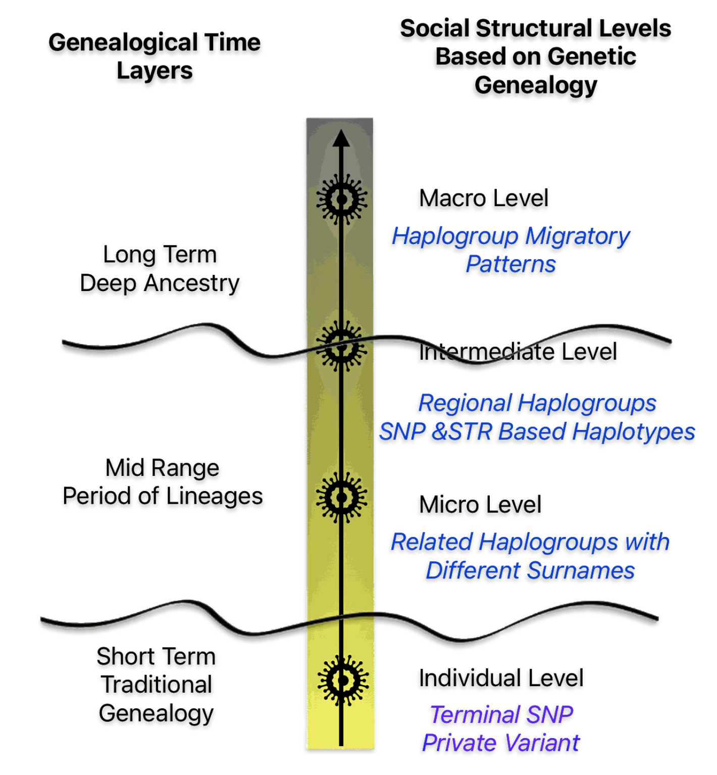
- Short Term – Normal Time: This is the realm of traditional genealogy and family history that spans roughly 300 years or 10 generations. I use 31 years are one generation. [1];
- Mid Range – Lineages: This middle layer of time can be viewed within a genetic genealogical perspective that focuses on Y-STR mutations. It is a period where surnames emerge. Using traditional genealogical methods with genetic genealogy can lead to promising leads on the location of haplogroup groups based on surnames and geographical areas. The middle historical time layer can be viewed in terms of tracing Single Nucleotide Polymorphisms (SNP) and Short Tandem Repeats (STR) Y-DNA mutations in lineage / clan groups and haplogroups.
- Long Range – Deep Ancestry: This is the foundational layer of genealogical time. It can provide an understanding of the correlation between haplogroup migration and geographical location. This time layer focuses on the correlation of genetic evidence with ancient cultural groups that existed in specific geographical areas and long-term climate and landscape changes as well as historic cultural geographical patterns across long stretches of time. This long range layer of time can be viewed within a genetic genealogical perspective that focuses on Y-SNP mutations;
Each of these layers of time are associated with differing orientations and sources of contextual background information to create family stories.
Reframing Contextual Factors for Mid Range and Deep Ancestry Time Layers
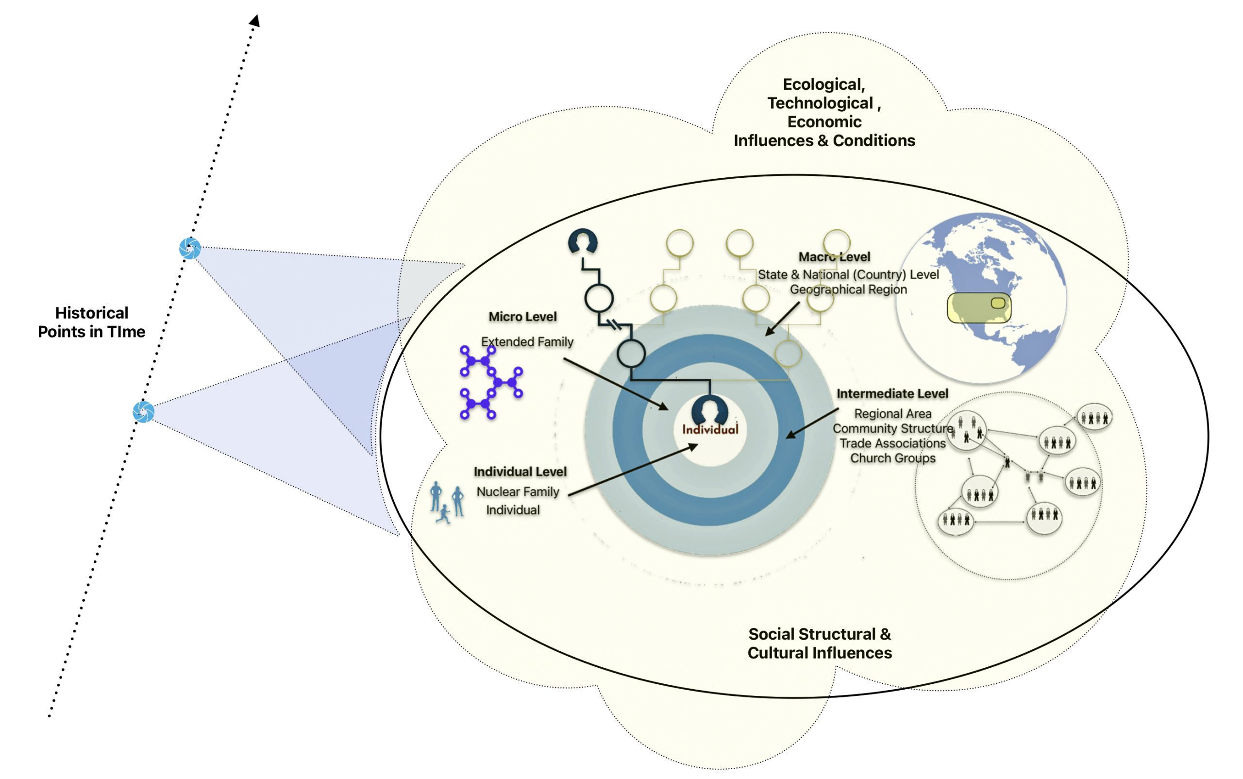
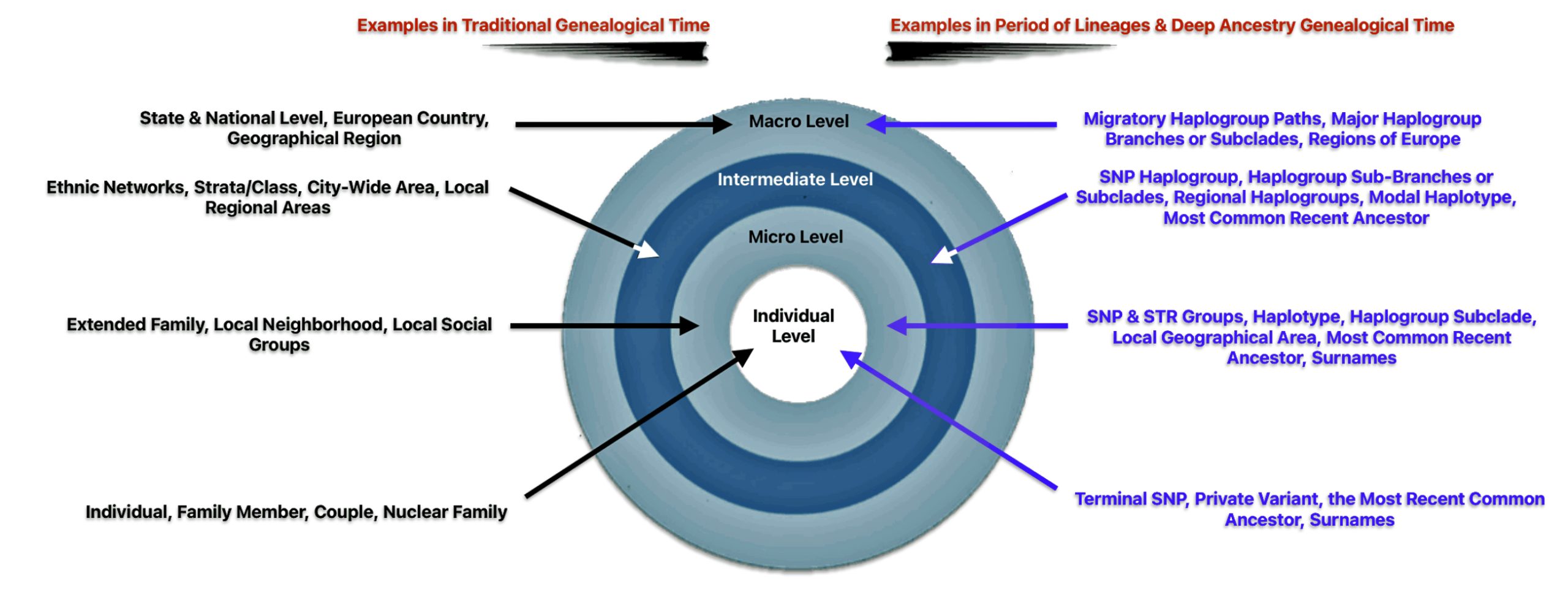
In the traditional genealogical time layer we have paper, digital and physical sources of historical evidence to create family stories. Contextual factors are broadly encapsulated in four social structural levels. (See table one.) They can help explain or provide descriptive information surrounding an ancestor or family’s life experiences in a particular time period.
Table One: Social Structural Levels or Networks of Influence in the Traditional or Short Term Genealogical Time Layer
| Social Structural Level | Examples of Social Structural Influences |
|---|---|
| Individual | Family Member / Couple Nuclear Family |
| Micro Level | Extended Family / Local Neighborhood Local Social Groups (Church, Local Community) Local Occupational Work Groups |
| Intermediate Level | Ethnic Networks Economic Strata / Class City-Wide area / Local Regional Areas |
| Macro Level | State and National Level European Country Geographical Region |
In addition to the various social structural levels that may play a prominent role in describing the experiences of ancestors and their families, there are ecological, technological, economic, cultural influences that may add historical context to the story. These influences may affect specific or all social structural levels, as illustrated below.
Illustration One: Time and Historical Context of Structure, Culture, and Other Factors in the Short Range Time Layer
As we move back in time, contextual evidence increasingly becomes associated with the intermediate and macrostructural levels. The ability to document these historical contextual factors of influence diminish as was we go back into the mid range and long range genealogical time layers. Evidence is not available for certain social structural levels and other contextual historical factors. This is illustrated in table two.
Table Two: Likelihood of Finding Information from Social Structural Levels Associated with Traditional Genealogy
| Time Period / Layer | Individual | Micro Level | Intermediate Level | Macro Level |
|---|---|---|---|---|
| Long Range – Deep Ancestry | X | X | ||
| Mid Range – Lineages | X | X | X | |
| Short Term – Normal Time | X | X | X | X |
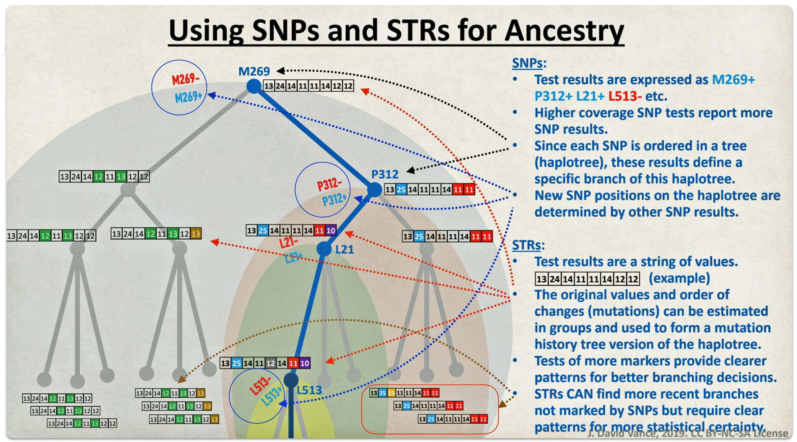
Our frame of reference shifts from individual ancestors and families to terminal single nucleotide polymorphisms (SNPs), short tandem repeats (STRs), the most recent common ancestor (tMRCA), haplotypes, haplogroup subclades, modal haplotypes and branches. [2]
Y-DNA SNP and STR mutations or mtDNA SNPs are the basic frames of reference for the mid range and long range time layers. These mutations help identify groups, based on those mutations, loosely akin to what are families in the short term or traditional time layer.
SNPs and STRs: The Underlying Connection Between the Three Time Layers
“In a nutshell, SNPs, single nucleotide polymorphisms, are the mutations that define different haplogroups. Haplogroups reach far back in time on the direct paternal, generally the surname, line. [3]
SNPs and STRs are the building blocks that tie the three genealogical time layers together. While both are part of each time layer, one can argue that SNPs characterize the long term genealogical time layer while STRs are provide a unique discriminatory power in the mid range or period of lineages genealogical time layer.
A Base Pair in DNA
Two complementary nitrogenous bases (adenine with thymine, and cytosine with guanine) that pair together to form the “rungs” of the DNA double helix, held together by hydrogen bonds. They are the building blocks of DNA structure where the sequence of these base pairs encodes genetic information.
Illustration Two: A Base Pair
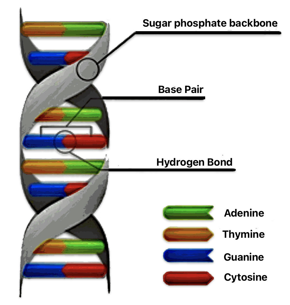
SNPs represent variations at a single DNA base position where one nucleotide in the DNA string is substituted for another. STRs are repeated sequences of DNA that consist of 2-6 base pairs occurring in a head-tail manner. For example, a sequence of DNA base sequences in the DNA chain resembling “GATAGATAGATAGATA” represents four repeats of the “GATA” pattern. These repeats can vary in length among different individuals, making them highly polymorphic (the occurrence of multiple distinct forms or variants). [4]
SNPs and STRs serve distinct purposes in genetic analysis across different time periods due to their unique mutation characteristics. STRs are ideal for recent genetic analysis (short range and mid range time periods) because they have a high mutation rate of approximately 10-3 to 10-4 per generation. [5] [6] This makes them particularly useful for population differentiation studies, genealogical matching within the past 500 years to 800 years, and forensic DNA testing and kinship analysis. [7] Completing a’ Big Y’ DNA test provides matches back 1,500 years. [8]
SNPs are better suited for studying ancient (long range) genetic history. They have extremely low mutation rates of approximately 10-8 . [9] They are considered “once in the lifetime of mankind” events. [10] They can effectively track population divergence dating back to the African exodus 50,000-75,000 years ago. [11] As more male individuals are tested, the SNP haplotrees can become more refined and identify sub branches or subclades in what I have identified as the mid range and short range time periods.
From a technical angle, SNPs work better with degraded DNA (e.g. ancients bones) due to smaller target regions. They also have greater mutational stability and require 40-60 loci to match the discriminatory power of 13-15 STRs. [12]
STRs provide higher information content per locus due to multiple alleles. (An allele is a variant form of a gene that occurs at a specific location (locus) on a DNA molecule.) They also can be used for high-resolution description of human evolutionary history. [13]
See my story: Y-DNA and the Griffis Paternal Line Part Three: The One-Two Punch of Using SNPs and STRs February 23, 2023
As indicated in illustration three below and discussed in a previous story, the “One-Two” punch of Y-DNA testing involves using the results of Y-SNP DNA tests to provide a general location of Y-DNA testers on the Y-DNA haplotree based on nested haplogroups. The ‘second punch’ uses Y-STR test results to help group test results within recent haplogroup branches and to assist in analyzing potential individual matches.
The analysis and comparison of individual Y-STR test results can help delineate lineages and tease out branches within the haplotree, fine-tuning relationships between people within the tree. The “One-Two Punch’ approach with SNP and STR data is particularly helpful in trasing out genetic ties with test results associated with different surnames and before the use of surnames in the period of lineages genealogical time layer.
Illustration Three: The Relationship Between SNPs and STRs in Refining Haplogroup Branches
While STR tests are used by individual testers to discover possible Y-DNA genetic matches with other testers, the results of STR tests can also provide insights into macroscopic demographic properties that can shed light on lineages and clans – well before the time of surnames. Y- STRs have a time window that runs back to the late Bronze Age.
“STRs … tell us about demography — specifically about bottlenecks and subsequent expansions, namely “founder events.” While SNPs tell us when they were created, STRs tell us about when the population burgeoned after a founding mutation. That SNP and STR clades have a fundamentally different interpretation has caused considerable confusion, but once understood, the methods are very useful complements.” [14]
STRs have been viewed as having limited use in estimating dates beyond about 50 to 100 generations (e.g. 1,550 – 3,100 years before present). However, there have been studies that indicate STR data can be utilized to for genealogical analysis into the Paleolithic era. (The Paleolithic period, also known as the Old Stone Age, generally spans from around 3.3 million years ago to approximately 11,650 years ago.) [15]
The Haplogroup and Most Recent Common Ancestor as the ‘Generation’ in the Mid Range and Deep Ancestry Time Layers
The concepts of an haplogroup and the Most Recent Common Ancestory (tMRCA) play a tandem role as defining what can be called a ‘generation’ in the deep ancestry and period of lineages genealogical time layers. However, pinpointing a ‘generation’ in the mid-range and long range time periods is not as exact as in the short range genealogical time layer.
“A haplogroup can be considered like an ancestor on your family tree. Each haplogroup forms a branch on that family tree. Depending on the age of the haplogroup (when it formed), you may have the name of that ancestor, or the ancestor may have lived so long ago that their name has been lost to time.
“Each haplogroup formed at a specific time and in a specific location. Testing of modern peoples and ancient DNA informs us of those locations and phylogenetic experts are able to build not just a tree of humankind, but also migration paths that those haplogroups took across and out of Africa and to the other continents.” [16]
A Y-DNA SNP mutation is akin to a direct paternal descendent. Haplogroups contain one or more unique SNP mutations. Each unique SNP mutation within the haplogroup pertain to a single line of descent. Each haplogroup originates from, and remains part of, a preceding single haplogroup.
“As such, any related group of haplogroups may be precisely modelled as a nested hierarchy, in which each set (haplogroup) is also a subset of a single broader set (as opposed, that is, to biparental models, such as human family trees). Haplogroups can be further divided into subclades.” [17]
There is at least one SNP mutation associated with a haplogroup. However, many haplogroups may have more than one SNP mutation associated with it, referred to as equivalents or equivalent SNPs.
“Equivalent SNPs” in a haplogroup refer to multiple SNPs that occur on the same genetic branch, essentially meaning they all indicate membership in the same haplogroup, even though they are slightly different mutations at the DNA level. Essentially they are considered the same for identifying a haplogroup as they all point to the same ancestral lineage within that group.
These SNPs are located on the same branch of the phylogenetic tree, indicating they arose around the same time in evolutionary history and are associated with the same haplogroup. It is often difficult to determine the exact chronological order of occurrence between equivalent SNPs. When multiple SNPs are tested, if they all show the same pattern (positive or negative for the same haplogroup), it strengthens the identification of that haplogroup. [18]
“Equivalent SNPs are variants that occupy the same branch as one another. This occurs when multiple SNPs are tested positive and negative for the same upstream and downstream SNPs and have all yielded the same positive and negative results from testers as the main SNP on the branch, making it impossible for our phylogenetic expert to confidently determine which of these variants are upstream or downstream of the others.” [19]
When multiple equivalent SNPs exist, they are often listed together in haplotrees and source documentation. Different laboratories and corporations may select different equivalent SNPs as their primary or defining marker for the same haplogroup.
In each nested genetic set of SNPs, there resides a ‘Most Common Recent Ancestor’. The determination of relationships of identified SNP mutations within the haplogroup relies on statistical methods like the rho statistic to estimate the time to most recent common ancestor (TMRCA), next-generation sequencing techniques that can identify SNPs in an unbiased way, and high-quality coverage of the Y chromosome to ensure accurate SNP identification. [20]
When dealing with equivalent SNPs in a haplogroup, the focus is not on choosing a single “most recent” common ancestor, but rather on understanding that these mutations represent the same ancestral point in the haplogroup’s history. The actual age estimation of the common ancestor is calculated using statistical methods and ‘molecular clock’ calculations rather than trying to determine which of the equivalent SNPs came first. [21]
In genetic genealogy, the most recent common ancestor (tMRCA) refers to the most recent individual from whom two or more people being tested are directly descended, essentially the point in time where their genetic lineages converge based on DNA analysis. The MRCA can be a specific person in a family tree, or a population-level ancestor estimated through genetic data analysis. Regarding the latter, the MRCA will often be represented by an estimated birth date and a statistical confidence level associated with the estimated date. [22]
Rob Spencer provides a cogent explanation of the relationship with tMRCA and when haplogroups are formed. Illustration four depicts an example of how the tMRCA and haplogroup formation dates can be different.
Illustration Four: Formation Dates of Haplogrups and tMRCA
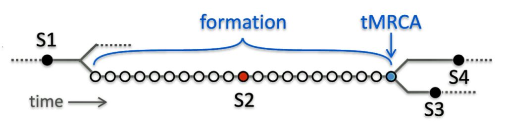
Spencer’s illustration focuses on the fact that the determination of when the MRCA emerged or was estimated to be born varies depending on who or what organization is calculating the MRCA date. The variation in estimates is also dependent upon the number of SNP mutations associated with a specific haplogroup.
“In a rapidly expanding population with many surviving lineages, tMRCA and formation are very close and may be identical. But for older and leaner lineages, a SNP may appear long before one of the originator’s descendants has two surviving lineages, and additional separate mutations may occur in that time. In the sketch, (illustration above), SNP S2 is one of 21 such equivalents: different mutations but evidently from a long unbranched line, since all DNA testers either have none of these 21 SNPs or they have all of them. The tMRCA for S2 is shown in blue; it’s where branches that have S3 and S4 split away. But the formation time for S2 cannot be directly measured and it could be anywhere between S2’s tMRCA and the previous tMRCA. YFull’s convention is to assign a SNP’s formation date to the previous SNP’S tMRCA (the left-most of the long run of equivalent SNPs). But it is perhaps better to estimate the formation date as halfway between, as shown by the red dot, which is what SNP Tracker does.” [23]
Different haplogroups exhibit substantial variation in their mutation rates. This can be due to bottlenecks or expansion in populations. Bottleneck events can create distinctive patterns that increase the rate of coalescence between lineages, lead to fewer overall haplotypes, and result in higher frequencies of the most common haplotypes. [24]
Different haplogroups may have undergone varying levels of genetic diversification based on their demographic history and population size. Migration patterns can create unique combinations of variants. [25] Some haplogroups have experienced more mutations over time due to geographic isolation leading to distinct mutation patterns, larger population sizes allowing more opportunities for mutations to occur, and older lineages having more time to accumulate variants. [26]
The age of population splits affects variant distribution. Older lineages have had more time to accumulate variants. Recent demographic events (5,000-10,000 years ago) particularly shape the distribution of rare variants. Population-specific variants can arise either from new mutations within a population or from the loss of variants in other populations [27]
The impact of growth on SNP variant diversity is particularly evident in founder populations, where initial small population sizes followed by rapid expansion create unique patterns of genetic variation and haplogroup distribution [28]
Differences between ‘Generations’ and ‘Haplogroups’
The parallel between ‘generation’ in the traditional genealogical time layer and ‘haplogroup’ in the other two time layers is limited. A family is associated with a specific network of individuals that can be associated with a ‘generation’. A generation is a group of people born around the same time and generally in the same area. A generation is also the average period of time it takes for children to be born, grow up, become adults, and have children. [29]
A haplogroup, on the other hand, is a group of people with similar genetic SNP and STR markers that can be traced back to a common ancestor. That common ancestor could have lived thousands of years before the group of people identified as having similar genetic markers. Despite the limited similarity between the terms family and haplogroup, their similarity is based on their ability to connect and trace patrilineal or matrilineal connections across each of the three time layers.
Illustration five below provides an example of comparing ‘generational’ and ‘haplogroup’ properties based on my genealogical evidence. On the left hand side of the illustration is eight generations depicting my patrilineal family lineage through traditional genealogical research. To the right of my traditional patrilineal lineage is my ‘recent’ genetic genealogical lineage depicted through haplogroups based on SNP mutations along my patrilineal line.
As reflected in the illustration, my traditional patrilineal genealogical tree depicts eight generations between fathers and sons. Generations can be viewed as the years between father and son. In this instance, generations range from 21 years to 41 years. My patrilineal line of descent, which comprises eight generations back, spans 217 years.
Illustration Five: Comparison of Generations in a Traditional Family Tree and ‘Genetic Generations’ in a Haplotree
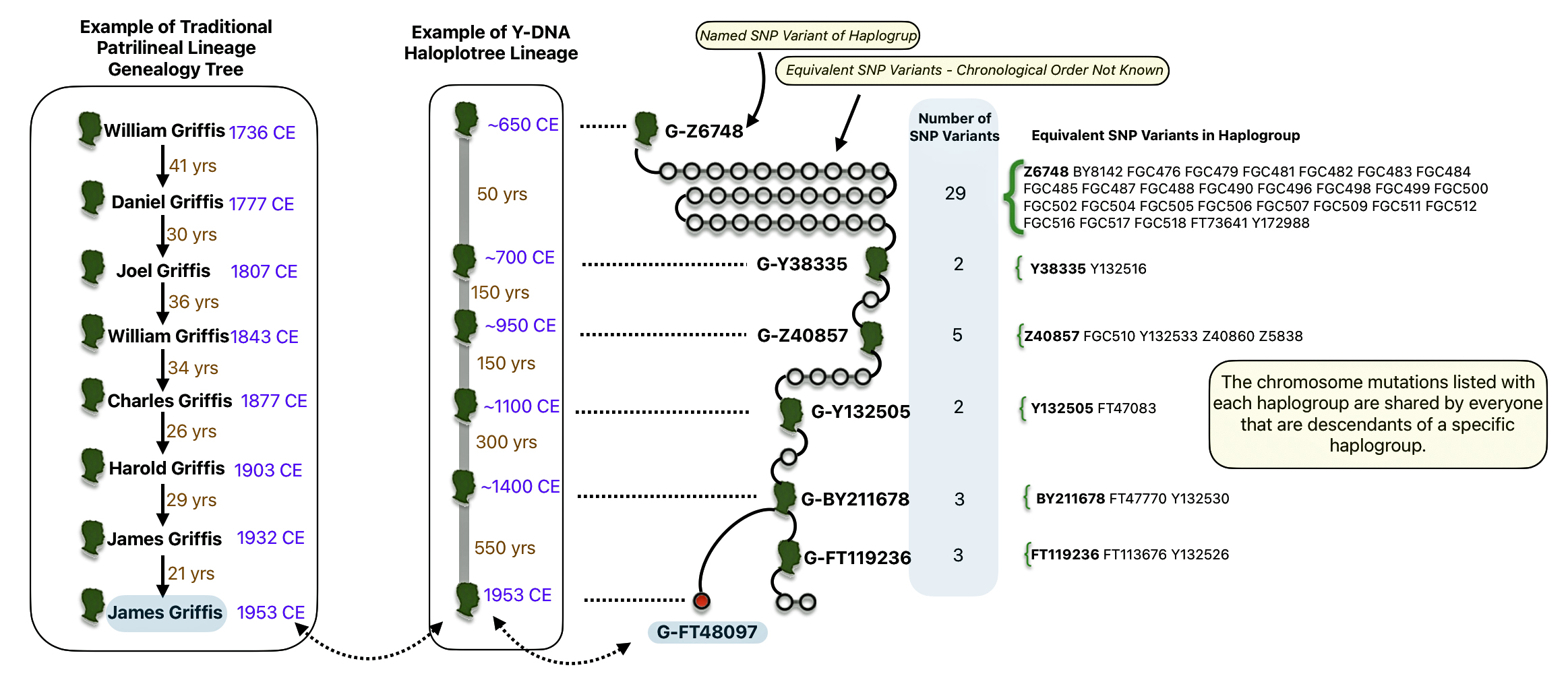
The recent haplogroups or ‘genetic generations’ in my patrilineal line, as reflected in illustration four, comprise five SNP mutation levels or ‘genetic generations’ prior to my terminal YDNA SNP which is identified as G-FT48097. There is another haplogroup that split off of my most recent haplogroup G-FY211678 that I am related to and is idenified as G-FT119236. I am not directly related to the G-FT119236 haplogroup.
As depicted in table three, three things are particularly notable with haplogroups: the range of years between each haplogroup, the variance of the number of SNPs associated with each haplogroup and the number of immedite descendants or subbranches for each haplogroup. The number of years that are between each haplogroup range from an estimated 50 years to 1400 years. The number of SNPs associated with each haplogroup vary greatly. A third observation, not evident in illustration five, is the number of branches or subclades – the number of male descendants from each haplogroup.
Table Three: SNP Variants and Immidiate Male Descendants Associated with Selected Haplogroups
| Haplogroup | Number of Associated SNPs | Estimated Years Between Haplogroup | Number of Phylogenetic Subclades |
|---|---|---|---|
| G-Z6748 | 29 | – – | 2 |
| G-Y38335 | 2 | 50 | 2 |
| G-Z40857 | 5 | 150 | 4 |
| G-Y132505 | 2 | 150 | 4 |
| G-BY211678 | 3 | 300 | 2 |
| G-FT48097 | – – | 500 |
Corresponding to the same time frame as table three, illustration six depicts a phylogenetic tree of haplogroups and subclades or branches that are associated with my ‘recent’ genetic descendants from haplofgroup G-Z6748.
Illustration Six: Phylogenetic Trees of Haplogroups Descending from G-Z4768
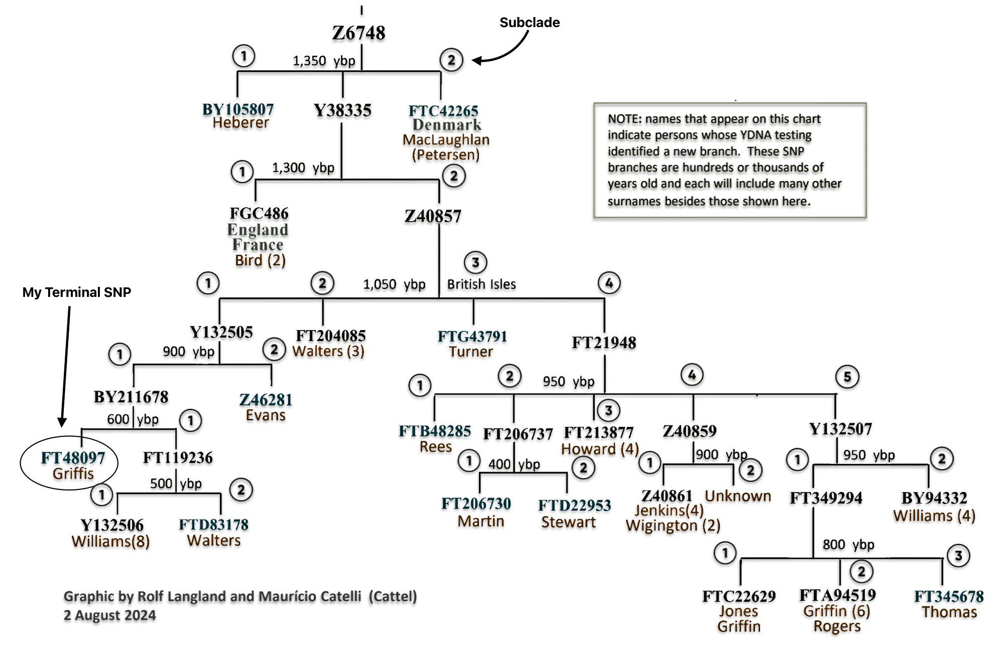
Table four illustrates the wide variance in estimating the year of birth for each of the common ancestors associated with each haplogroup. While individual dates should be interpreted cautiously, collectively they can provide reliable benchmarks. Most genealogists recommend using 95% confidence intervals for the most accurate interpretation of results. Sixty-eight percent confidence intervals are recommended for narrower, but less certain estimates [30]
Table Four: The Most Recent Common Ancestor (tMRCA) Associated with Each Haplogroup
| Haplogroup | Estimated Birth Date of tMRCA | 95 % Confidence Range of Birth | 95% Confidence in Yrs | Rounded Estimate of tMRCA Birth Date |
|---|---|---|---|---|
| G-Y38335 | 708 CE | 425 – 943 CE | 518 yrs | 700 CE |
| G-Z40857 | 970 CE | 737 – 1162 CE | 425 | 950 CE |
| G-Y132505 | 1115 CE | 841 – 1332 CE | 491 | 1100 CE |
| G-BY211678 | 1413 CE | 1210 – 1571 CE | 361 | 1400 CE |
The reliability of Y-DNA SNP-based MRCA estimates varies significantly depending on the timeframe and methodology used. For genetic genealogy purposes, the accuracy varies by depth of time. For prehistoric migrations for about 5000 years, there is a variance of 500 years in precision. For MRCA’s within 200 years, it is estimated that he variance could be around a 30 year variance. For MRCA dating based on cultural origins within 800 years, the precision of the estimate is plus or minus 500 years. [31]
Different testing companies use varying mutation rates. YFull utilizes 144.4 years per SNP. FamilyTreeDNA results associated with the BigY500 DNA test utilized : 131.3 years per SNP. For the BIig Y 700 Y-DNA test, a mutation rate of 83.3 years per SNP is used. [32]
Haplotrees as Family Trees in the Mid Range and Long Term Genealogical Time Layers
A haplotree is a branching diagram that shows the evolutionary relationships and genetic ancestry of human populations through inherited genetic markers. These trees represent the journey of human genetic lineages and help visualize how different groups are related to each other genetically. [33] There are two main types of haplotrees: Mitochondrial DNA (mtDNA) haplotrees that track maternal lineages through mitochondrial DNA and Y-DNA haplotrees that track paternal lineages through Y chromosome mutations.
Haplotrees follow a nested hierarchical structure where each haplogroup originates from and remains part of a preceding haplogroup. They are typically labeled using alphabetical nomenclature, starting with an initial letter followed by numbers and additional letters for refinements (e.g., A → A1 → A1a). [34]
The Y-DNA haplotree is particularly dynamic, with new branches being added frequently as more genetic data becomes available. As of recent updates, it has grown significantly from its initial 153 branches and 243 Y-SNPs to encompass thousands of documented genetic lineages. [35]
As of February 2024, it was claimed that the Y-DNA haplotree contains 76,626 distinct branches (as of February 2024). [36] Another source indicates by the end of 2024, these totals grew to 86,892 branches and 734,748 variants, marking a full-year increase from 2023 of 11,823 branches (15.5%) and 83,752 variants (12.9%). [37]
Unlike the Y DNA tree, which is defined and constructed by the genetic community, new mitochondrial DNA branches cannot be added to the official mitochondrial Phylotree. The official mitochondrial Phylotree is maintained at www.phylotree.org and is periodically updated. The most recent version is mtDNA tree build 17, published and updated in February 2016. [38]
Haplotrees are built on the principle that genetic mutations accumulate and remain fixed in DNA over time. When a mutation occurs, all descendants of that individual will carry that genetic marker. The sequential nature of these mutations allows scientists to reconstruct the historical order of genetic changes and map human migrations throughout history.
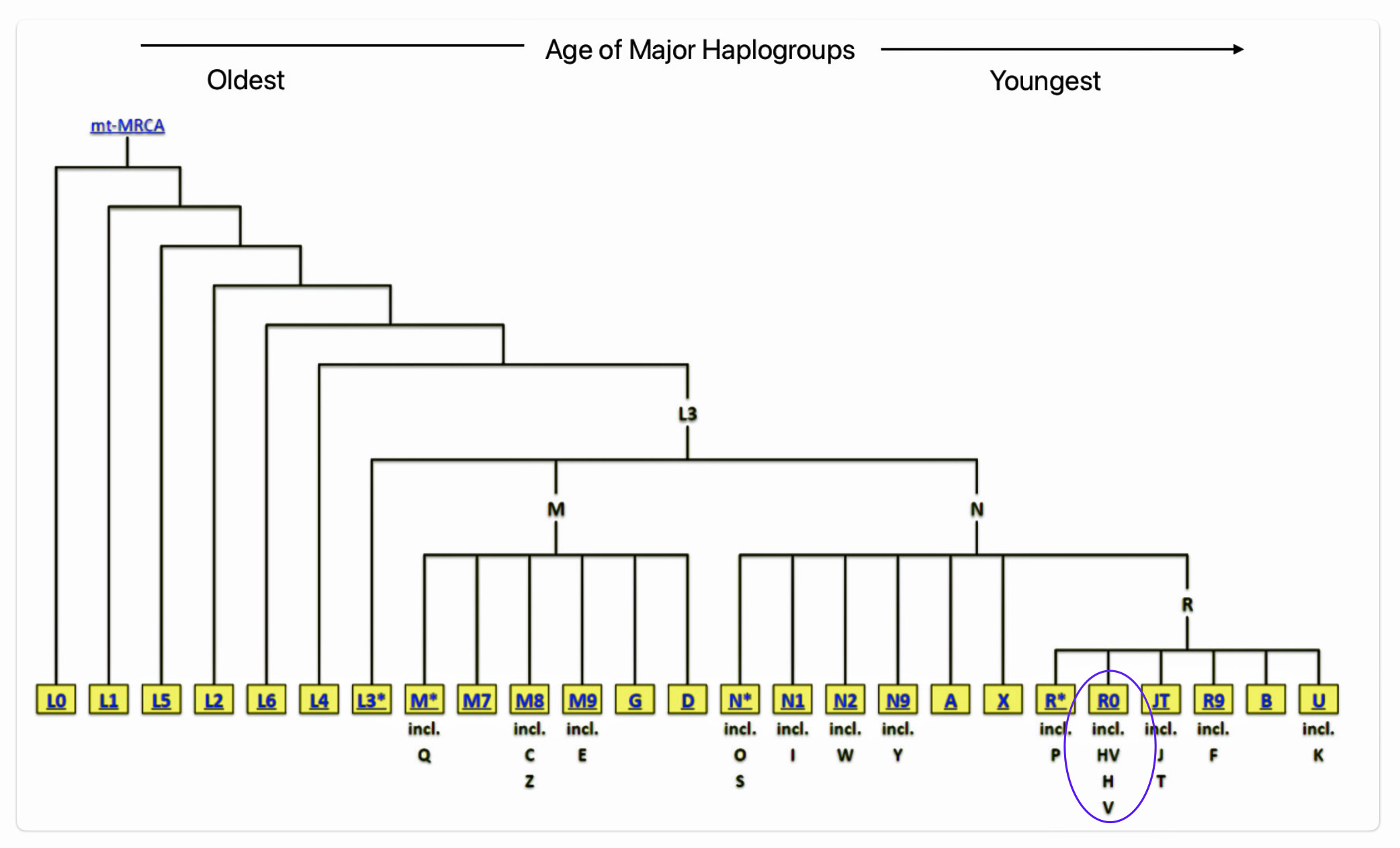
Illustration seven depicts the major branches for the Y-DNA haplogroup tree and illustration eight depicts the major branches for the mtDNA maternal lineages .
Illustration Seven: Major Branches of the Y-DNA Haplogroup Tree
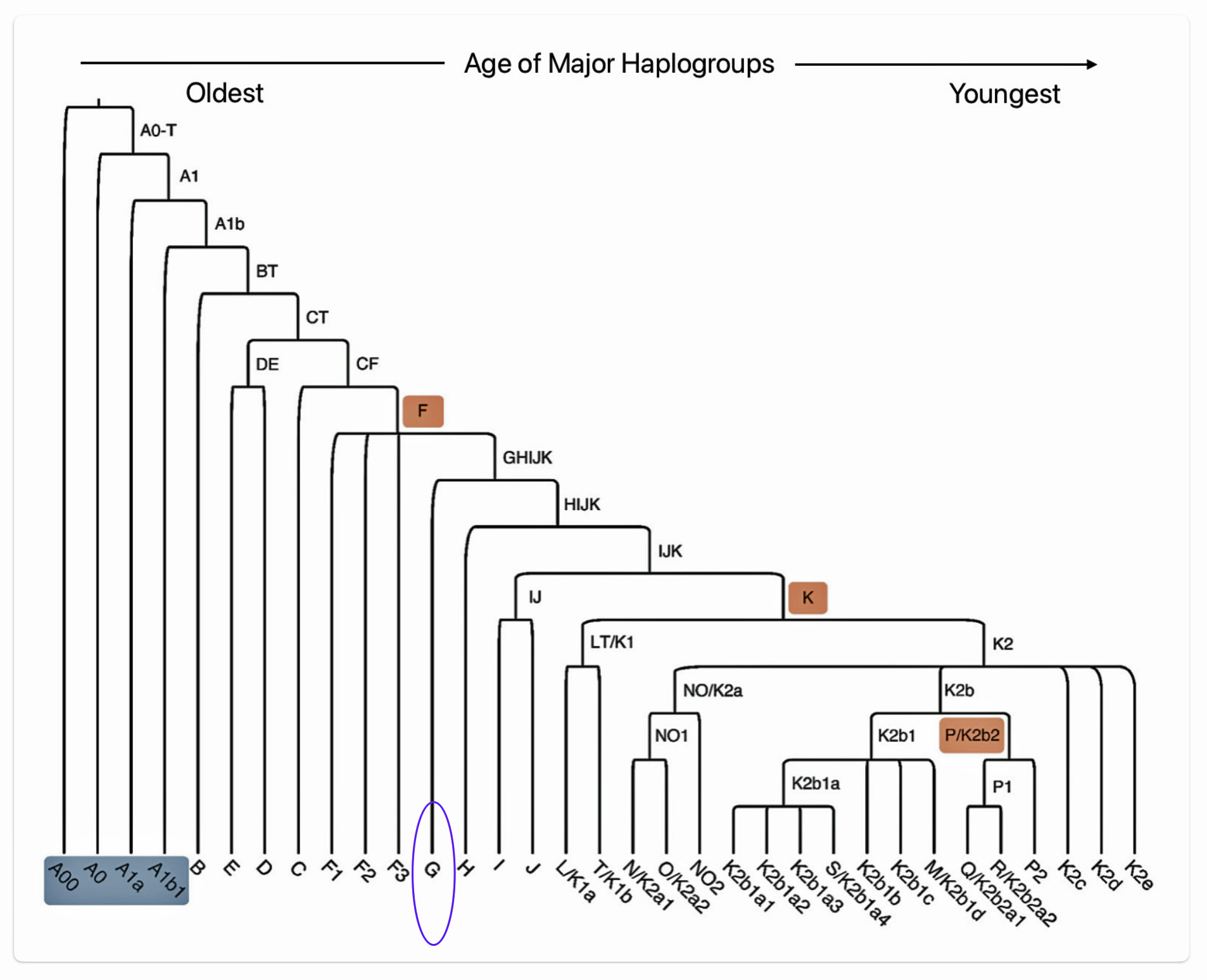
Illustration Eight: Major Branches of the mtDNA Haplogroup Tree
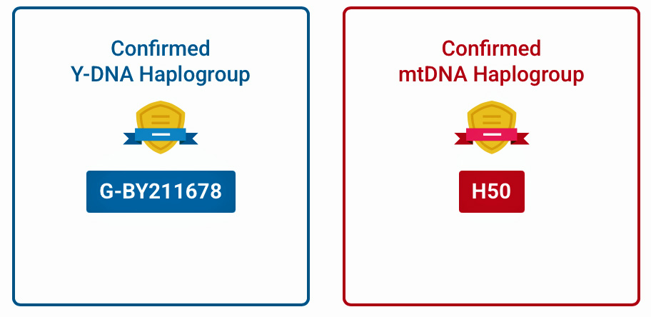
We can look at my DNA results in the context of haplotrees. Results of my FamilyTreeDNA (FTDNA) Y-700 DNA test indicate my Y-DNA terminal haplogroup is G-BY211678 and my mtDNA phylotree is H50.
The relative positions of these results are indicated in illustrations nine and ten of the major haplotree branches by blue circles.
Given the specificity and the wide range of SNPS tested in the Y-700 DNA test, my results reflect a new terminal end point, FT-48097 in the G -BY211678 branch of the G Haplotree. [38] A terminal SNP represents the furthest known branch or “leaf” on haplotree tree. (See Illustration nine.)
This metaphorical tree framework has proven so useful that it has become a standard way to visualize and understand Y-DNA testing results, with modern genetic testing companies like Family Tree DNA adopting it as their primary way to represent genetic relationships.
Illustration Nine: The Tree Metaphor for explaining Branches in the G Haplotree Branch and My Test Results
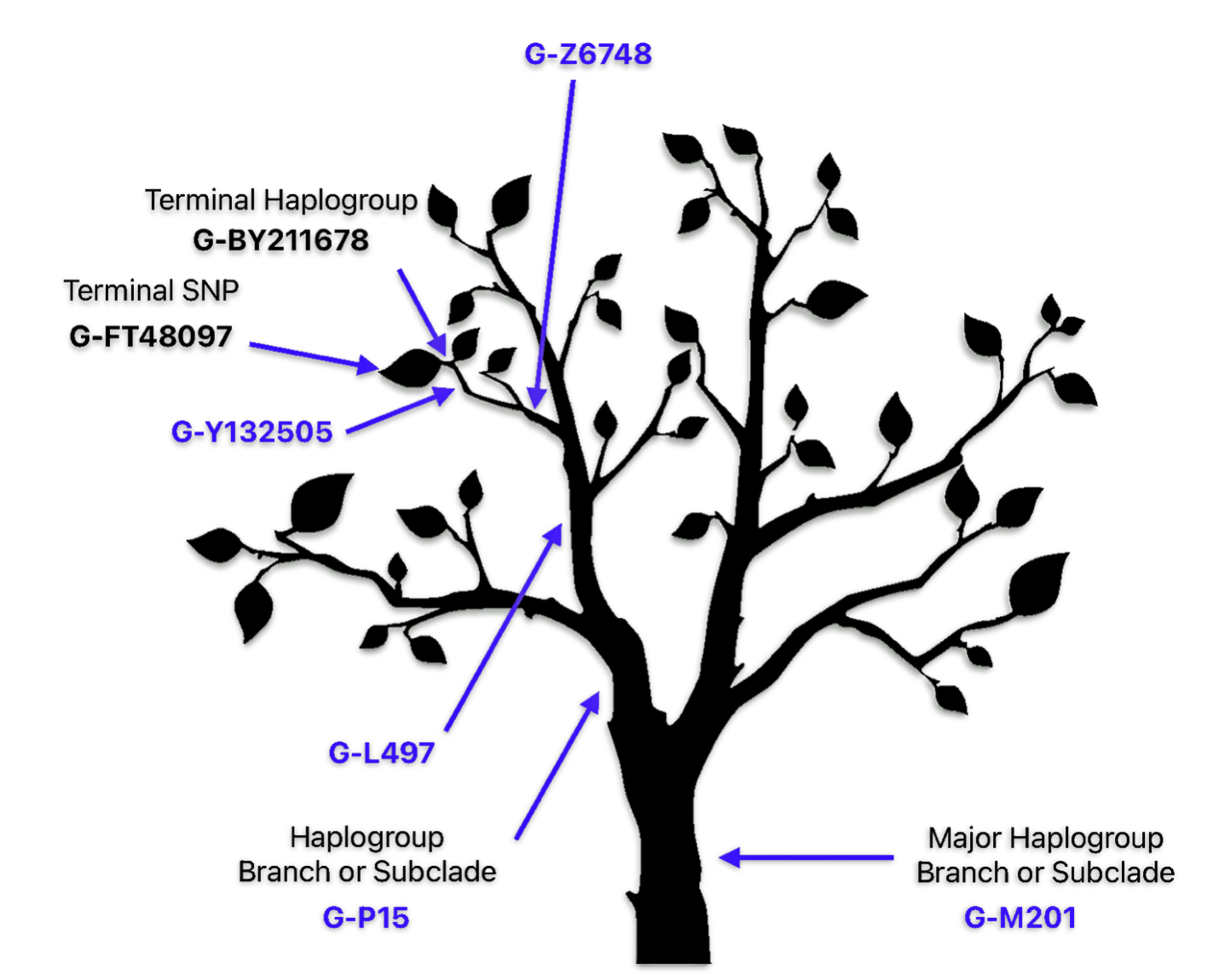
The application of the tree metaphor specifically to terminal SNPs emerged from the broader field of genetic genealogy and haplogroup identification. A terminal SNP represents the furthest known branch or “leaf” on a person’s genetic tree. This modern usage combines the traditional tree metaphor with current genetic science and the branch structure of the DNA haplotree. The main branches or subclades represent major haplogroups. Smaller branches indicate subgroups. The terminal SNP represents the smallest “leaf” on the branch.
Unlike Y-line DNA, no additional SNP tests are required to fully determine one’s mitochondrial DNA haplogroup. The full mitochondrial sequence test (mtFullSequence) at FTDNA provides the most detailed, full haplogroup designation. With the HVR1 (mtDNA) and HVR2 (mtDNAPlus) tests, you receive a base haplogroup. The full sequence is required to determine your full haplogroup.
“To put this in perspective, think of your mitochondrial DNA as a clock face. There are a total of 16,569 locations in your mitochondrial DNA. The HVR1 test tests the number of locations from 11:55 to noon and the HVR2 test tests the number of locations between noon and 12:05PM. The full sequence test tests the rest, the balance of the 50 minutes of the hour.” [39]
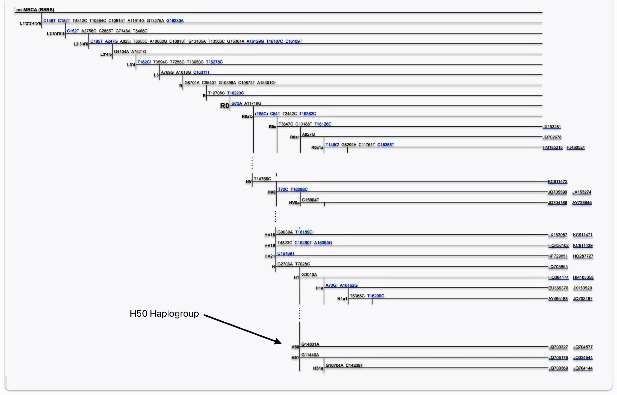
Illustration Ten: The H50 Branch on the mtDNA PhyloTree
Reframing Contextual Factors for Mid Range and Deep Ancestry Time Layers
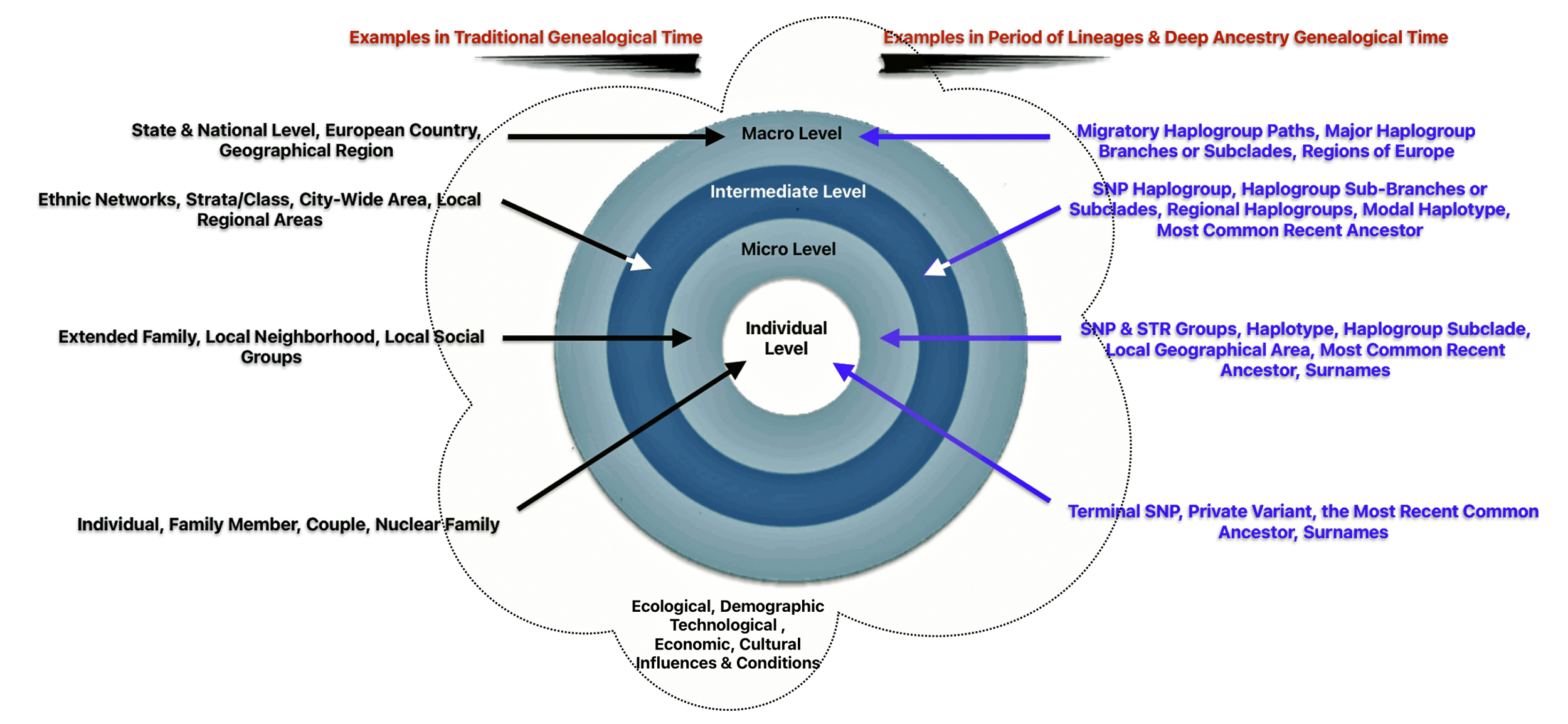
Given the change in the frame of reference in developing family stories in the mid and long range time periods, it is more useful to redefine the four ‘social’ structural levels of influence in genetic genealogical terms, as indicated in table five.
Table Five: Comparison of Structural Influences between Different Genealgical Layers of Time
| Social Structural Level | Examples in Short Term Time Layer | Examples in Mid Range & Long Range Layers |
|---|---|---|
| Individual | Family Member; Couple; Nuclear Family; ‘A generation’ | Terminal SNP; Private Variant; the Most Recent Common Ancestor (tMRCA) |
| Micro Level | Extended Family; Local Neighborhood; Local Social Groups | SNP & STR Groups; Genetic Distance; Haplogroup subclade; Modal Haplotype; tMRCA Localized Geographical Area |
| Intermediate Level | Ethnic Networks; Strata / Class; City-Wide area; Local Regional Areas | SNP Haplogroup Sub-branches / Subclades; Modal Haplotype;; tMRCA Regional Geographic Area |
| Macro Level | State & National Level; European Country; Geographical Region | Migratory Paths of Haplogroups; Major Branches of Haplogroups; tMRCA; Regions of Europe |
The ‘individual‘ level in the mid range and long term levels of time are ideally represented by a terminal SNP or private variant. A terminal SNP is the defining mutation that represents the most recently known branch on a Y-DNA haplogroup tree, an haplotree. A private variant is a genetic mutation that has occurred in a specific family line but has not yet been found in other tested individuals. These variants represent new SNPs that are unique to particular lineages. [40]
“New branches emerge when a variant not only becomes a Named Variant but also fulfills additional criteria: at least one person must test negative for it. This “negative test” helps distinguish the new branch from equivalent ones, signaling a point of divergence in the tree. Each branch represents a distinct lineage, connecting individuals to their unique paternal heritage and further refining our understanding of the tree’s structure.” [41]
There are distinct differences between private variants and terminal SNPs. When a private variant is found in enough testers and receives official designation, it can become a new terminal SNP for those who carry it. This demonstrates the evolving nature of genetic genealogy classification as more people test their DNA.
The ‘micro‘ level is represented by haplogroup subclades or branches that are related to the terminal SNP or private variant. The subsclades are in a ‘local’ geographical area and are related to a common ancestor that resided in that geographical area. It is analogous to the ‘extended family’ or ‘local social groups’ . This is the genetic social structural level that can reveal the emergence of surnames in the period of lineages.
Illustration Eleven: Genealogical Time and Social Structural Levels
The ‘intermediate‘ level straddles the mid range and long range time layers of genealogical time. The social structures in this time layer are akin to ‘ethnic networks’ or larger networks and haplogroups based in ‘regional geographical areas’. It is represented by a larger portion of haplogroup subclades which comprise haplogroup branches that have a common genetic ancestor that migrated from one geographical area to another. The Phylogenetic tree of haplogroups descending from G-Z4768 in illustration six above would be an example.
The ‘macro‘ level is in the long range genealogical time layer. It is graphically reflected by the migratory paths of major branches in an haplogroup lineage. This time layer is similar to French historian Fernand Braudel’s “long duration”. It is a time layer which emphasizes studying history or genealogy through the lens of long-term, slow-moving structures like geography, climate, and demographics, rather than focusing on short-term events or individual figures. It is essentially looking at the deep, underlying patterns of history that persist over extended periods of time, often beyond human memory. [42]
Illustration twelve depicts the differences in the social structural levels in each of the three genealogical time layers.
Illustration Twelve: Historical Context of Social Structure in the Three GenealogicalTime Layers
The three layers of genealogical time rely upon different methods of gathering contextual evidence. I have discussed contextual factors found in the traditional or short term genealogical time layer in a previous story.
As depicted in illustration thirteen, in addition to the various social structural levels that may influence our development of a story about a family member of family in the traditional genealogical time layer, there are ecological, technological, economic, cultural influences that may add historical context to the story. These influences may affect specific or all social structural levels. Rather than delve into possible relationships of causation, I have simply recognized the impact of and interplay between social, cultural, technological influences when weaving stories from our genealogical evidence.
Illustration Thirteen: Social Structural Levels and Other Influences in the Three Genealogical Time Layers
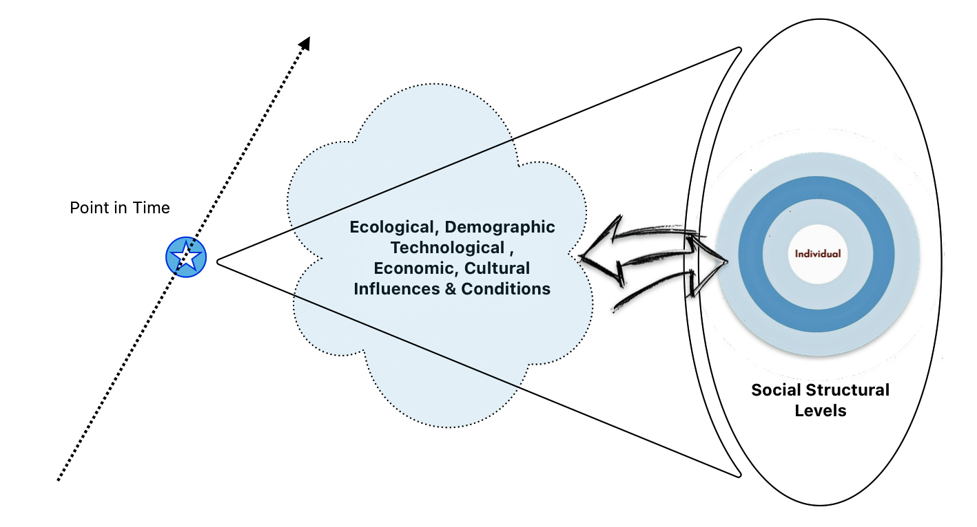
The long term and mid range ancestry genealogical time layers are also influenced by contextual factors. However, the ability to retrieve evidence on these factors diminishes as one goes back in time. These contextual factors in the period of deep ancestry are largely the outcome of a series of environmental, demographic and evolutionary events reflected in migration, genetic bottlenecks, founder events, admixture, population isolation, natural selection and genetic drift which occurred in different parts of the world at various time points in history. [43]
In human populations, changes in genetic variation are driven not only by genetic processes themselves, but can also arise from environmental, cultural or social changes. SNPs and STRs are influenced by several key factors that affect their occurrence and distribution throughout the genome. Demographic population patterns significantly influence SNP and STR mutation patterns through several key mechanisms.
Rob Spencer’s research in genealogy, particularly regarding “bottleneck” events, focuses on identifying periods in a population’s history where a significant decrease in population size occurred, which can leave a noticeable genetic signature in the genealogical record and impact the diversity of descendants today. Conversely, a founder event happens when a small group separates from a larger population to establish a new colony. [44]
“Cultural factors and processes can influence migration patterns and genetic isolation of populations, and can be responsible for the patterns of genetic variation as a result of gene-culture co-inheritance (e.g. a preference of cousin marriage). Understanding how social and cultural processes affect the genetic patterns of human populations over time has brought together anthropologists, geneticists and evolutionary biologists, and the availability of genomic data and powerful statistical methods widens the scope of questions that analyses of genetic information can answer.” [45]
The long term and mid range ancestry genealogical time layers rely on paleo-genomic, anthropological sources and historical analyses of cultural groups for contextual evidence. [46] The contextual sources for the deep ancestry time period are discussed in part three of this series of stories.
Illustration Fourteen: Historical Context of Social Structure, Culture, and Other Factors in the Three Genealogical Time Layers
A Illustrative Model for Depicting the Mid Range and Long Term Genealogical Time Periods
Examples for each of the four structural levels in mid and long range genealogical time are provided in an illustrated model of genealogical time and historical contexts of structural and cultural factors below.
Illustration Fifteen: Time and Historical Context of Structure, Culture, and Other Factors in the Mid and Long Range Genealogical Time Layers
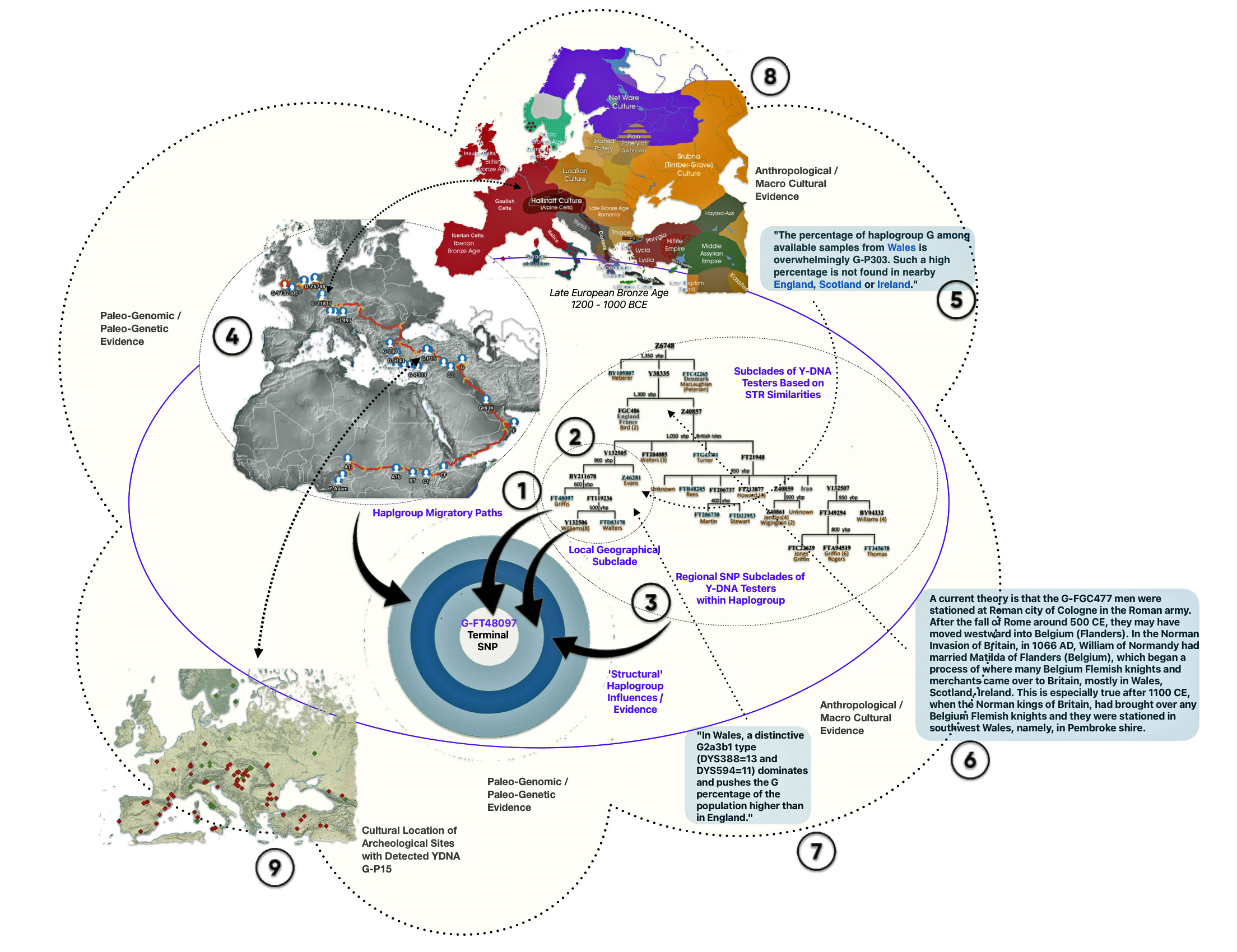
The examples for each of the social structural levels in the illustration are based on my genetic genealogical past. The examples for creating the illustration are from various sources. [47]
| Reference Number in Model | Structural Level | Example |
|---|---|---|
| One | Individual | My terminal SNP G-FT480 based on Y-700 FamilyTreeDNA results |
| Two | Micro | Phylogenetic Tree of Decendents of Haplogroup G-Y132505 |
| Three | Intermediate | Phylogenetic Tree of Decendents of Haplogroup G-Z6748 |
| Four | Macro | Migratory Path of G Haplogroup in Europe |
Reference Number 2 & 3 in the Model
The Phylogenetic tree is based on the current YDNA descendants of Haplogroup G-Z6748.
A subset of the phylogentic tree, which represents the micro level, is the haplogroup G-Z6748. This haplogroup appears to be a largely Welsh haplogroup, though extending into neighboring parts of England.
My Y-700 DNA test results as reflected in work compiled by the project administrators of the FamilyTreeDNA G-L497 work group project. [48]
Reference Number 4 in the Model
An illustrative example used in the model depicted above for the macro social structural level is a depiction of the general migratory path for my patrilineal genetic ancestors through the G-L497 haplogroup line. The ‘reconstructed’ migratory path was created using Globetrekker.
Globetrekker is an innovative DNA mapping tool launched by FamilyTreeDNA (FTDNA) in July 2023. The mapping tool visualizes paternal ancestry migration paths. This feature is only available to customers who have taken the Big Y-500 or Big Y-700 test. [49]
Reference Number 5 & 7 in the Model
An observation is noted in the illustrated model about the high percentage of population in Wales that exhibit STR values associated with the G-P303 haplogroup. “In Wales, a distinctive G2a3b1 type (DYS388=13 and DYS594=11) dominates there and pushes the G percentage of the population higher than in England.” In the model, it is used to illustrate a micro level genetic observation that is found in the short term and mid level genealogical time layers.
“In Wales, a distinctive G2a3b1 type (DYS388=13 and DYS594=11) dominates and pushes the G percentage of the population higher than in England.“
DYS stands for DNA Y-chromosome Segment. It is used to describe a segment of DNA on the Y chromosome that contains short tandem repeats (STRs). STRs are short DNA patterns that repeat in a specific sequence. All STRs are given a unique identification number. For example, DYS388: the D indicates that the segment is a DNA segment, the Y indicates that the segment is on the Y chromosome, the S indicates that it is a unique segment, and the number 388 is the identifier.
The values for the two abovementioned DYS’s are uniquelyassociated with the Haplogroup G-P303 (G2a2b2a, formerly G2a3b1).
Reference Number 6 in the Model
This observation is associated with the intermediate structural level. It is a current theory proffered by a member of the FamilyTreeDNA working project group for the Z-6748 Haplogroup. The YDNA tests associated with this group have ancestors that appear to have come from Wales.

The current theory is the ancestor of this YDNA line came across the English Channel with the Normans around the Norman Invastion. While the ancestor was not Norman he was probably a French or Belgium.
Reference Number 8 in the Model
Examples of contextual evidence from macro cultural and paleo-genomic research are correlated with each of the four structural levels. This is an example of macro-cultural contextual evidence in illustration three provides a map of cultural groups around 1,000 – 1,200 BCE.
The information in the map is correlated with when the G-Z1817 haplogroup existed in Europe. The haplogroup follows an ancestral path that descended from earlier G lineages that were present in the region approximately 4,550 BCE. The haplogroup emerged from the G-CTS9737 haplogroup around 3,050 BCE during the transition between the Stone Age and Metal Ages.
Example of Cultural Groups in Europe Around 1000 1200 BCE
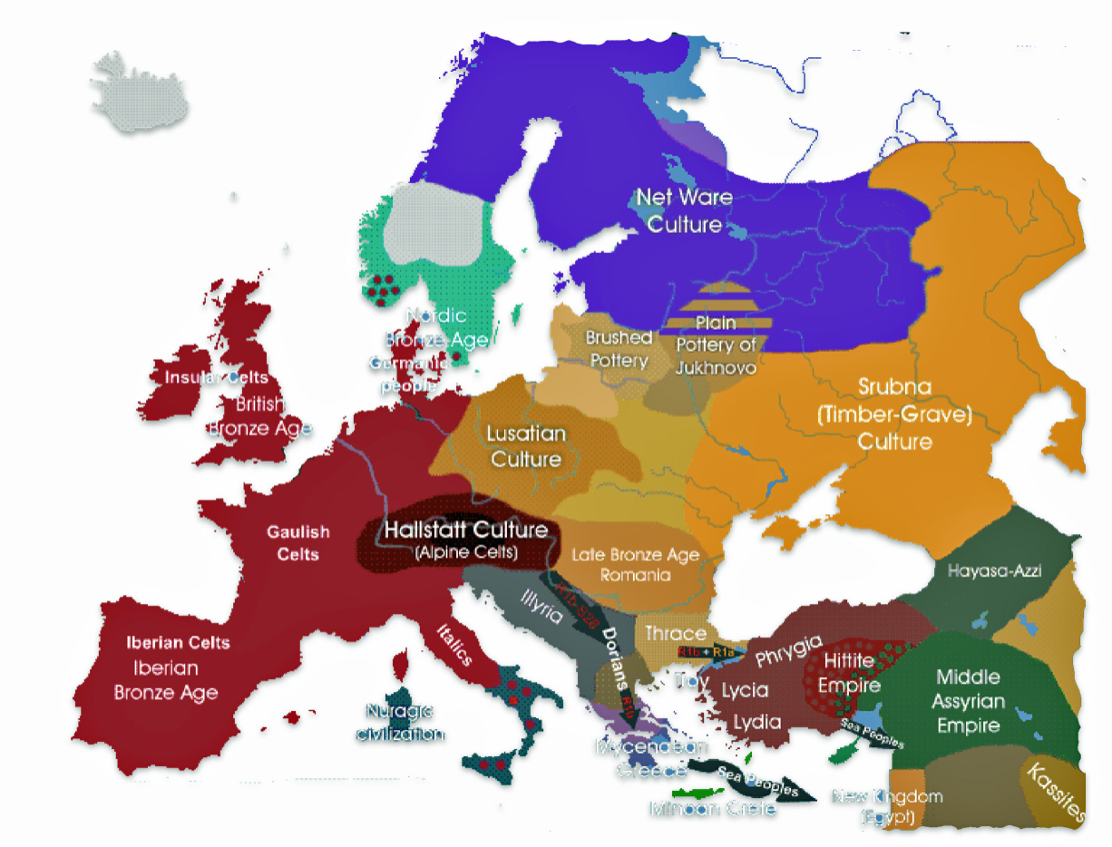
The haplogroup appears to have a predominantly Germanic and Central European focus, with its distribution suggesting possible connections to early Germanic populations. The modern pattern indicates the haplogroup likely played a role in Central European population movements, though maintaining its strongest presence in German-speaking regions. [50]
Reference Number 9 in the Model
Ths is an illustrative example at the macro level provides a correlation of where ancient DNA (aDNA) remains have been found that were part of the G-P15 haplogroup. G-P15, also known as haplogroup G2a, is a Y-chromosome haplogroup that emerged approximately 15,000-16,000 years ago.
Example of G-P15 Ancient remains in Europe
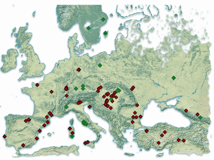
This genetic lineage is defined by specific mutations on the Y-chromosome, particularly the P15 marker. The G-P15 haplogroup is an ancestral group of my more historically immediate haplogroups. Current research indicates that G-P15 represents one of the main Neolithic genetic links connecting early farmers who migrated across different European routes, including the northern route through the Balkans to Central Europe and the western maritime route to the Western Mediterranean. [51]
Weaving Genealogical Stories Across the Three Layers of Time
This story provdes a model to explain the connectiveness of three different genealogical time layers and associated contextual sources of evidence for developing genealogical stories. The combination of traditional genealogical research with genetic genealogical analysis offers several powerful benefits for extending research through three layers of genealogical time. While the terminology, the objects of research and reseach methods are differenet, there is coherence between the two approaches to tie family history across the time layers. Haplogroup testing can help overcome genealogical dead ends or birckwalls by offering clues about ancestral origins beyond documented records, providing direction for research when traditional records are unavailable, and connecting genetic matches who share common ancestors.
Haplogroups enhance location-based research. They point to specific geographic regions where ancestors lived. They can confirm family origins and migration patterns. They also provide insights about ancestral locations from thousands of years ago that are not documented in historical records.
The combination of research through the three genealogical time layers helps validate genealogical research. DNA testing can confirm or disprove suspected family connections. Haplogroups can verify heritage claims that are too distant for autosomal DNA testing or beyond the reach of traditional research. Y-DNA patterns can help confirm surname connections and lineages.
The combination research across the three time layers provides a deeper historical understanding by revealing ancient migration patterns of family lines. It connects family history to broader historical movements. It provides insights about ancestors’ lives thousands of years before written records.
Each time layer provides valuable clues and they should be used as a unique source of evidence in our genealogical research.
Source:
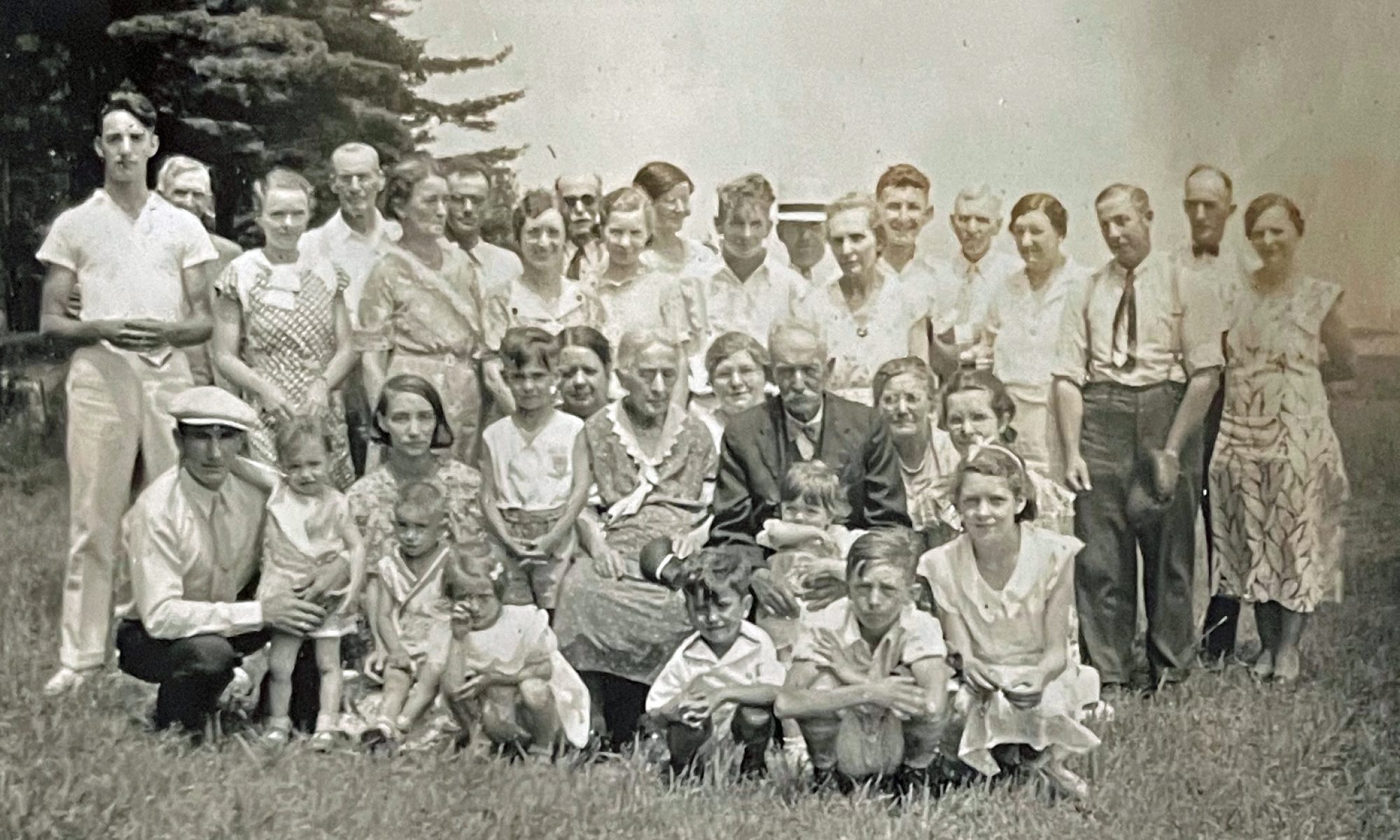
Feature Banner: The banner at the top of the story is a depiction of the two models associated with the three layers of genealogical time with the four social structural levels of historical context and other factors. .
[1] I have used 31 or 33 years as a rough estimate of a generation. This estimate has been ‘deduced’ after reading through the research and opinions about what is a generation in terms of years.
The conversion from generations to years typically uses a generation interval of approximately 30 years, rather than the previously assumed 20-25 years. This longer interval has been validated through extensive genealogical studies and population registers. For the mosst accurate calculations, it is recommended that an interval of 28-31.5 years be used.
Tremblay M, Vézina H. New estimates of intergenerational time intervals for the calculation of age and origins of mutations. Am J Hum Genet. 2000 Feb;66(2):651-8. doi: 10.1086/302770. PMID: 10677323; PMCID: PMC1288116, https://pmc.ncbi.nlm.nih.gov/articles/PMC1288116/
Also, see for example:
“But just how long is a generation? Don’t we all know as a matter of common knowledge that it generally averages about 25 years from the birth of a parent to the birth of a child. …
“I’ve shaded my earlier preferred number, 34, down a bit, to 33 or 32 but varying with the ethnicity, place, and period of the population.
“(Based on a study of family documentation) For a total of 21 male-line generations among five lines, the average interval was close to 34 years per generation. For 19 female-line generations from four lines, the average was an exact 29 years per generation.”
John Barrett Rob, How Long is a Generation?, https://www.johnbrobb.com/Content/DNA/How_Long_Is_A_Human_Generation.pdf
“For the Y chromosome these rates assume a 31 year generation.”
J. Douglas McDonald, TMRCA Calculator, Oct 2014 version, Clan Donald, USA website, Https://clandonaldusa.org/index.php/tmrca-calculator
“Our analyses of whole-genome data reveal an average generation time of 26.9 years across the past 250,000 years, with fathers consistently older (30.7 years) than mothers (23.2 years).”
Richard J Wang, Samer I. Al-Saffar, Jeffery Rogers and Mathew W. Hah, Human generation times across the past 250,000 years, Science Advances, 6 Jan 2023, Vol 9 Issue 1, https://www.science.org/doi/10.1126/sciadv.abm7047.
“Male-line generations, from father to son, are always longer on average than female-line generations, from mother to daughter. They show, too, that both are longer than the 25-year interval that conventional wisdom has assigned to a generation. The male generation is at least a third longer, the female generation is longer by perhaps half that amount.”
“(T)he accepted 25-year average has worked quite acceptably, and birth dates too far out of line with it are properly suspect.”
“As a check on those values, which are based on extensive data and rigorous mathematical analysis, although rounded off for ease of use, I decided to compare the generational intervals from all-male or all-female ranges in my own family lines for the years 1700 to 2000, and was pleasantly surprised to see how closely they agree. For a total of 21 male-line generations among five lines, the average interval was 34 years per generation. For 19 female-line generations from four lines, the average was 29 years per generation.”
“However, to convert generations to years and probable date ranges, use a value for the generational interval that is soundly based on the best currently available evidence.”
Donn Devine, How Long is a generation? Science Provides an Answer, International Society of Genetic Genealogy (ISOG) Wiki, This page was last edited on 16 November 2016, https://isogg.org/wiki/How_long_is_a_generation%3F_Science_provides_an_answer. This article was originally published in Ancestry Magazine, Sep-Oct 2005, Volume 23, Number 4, pp51-53.
Marc Tremblay et al., “New Estimation of Intergenerational Time Intervals for the Calculation of Age and Origin of Mutations,” American Journal of Human Genetics 66 (Feb. 2000): 651-658.
Nancy Howell calculated average generational intervals among present-day members of the !Kung tribe. The !Kung are a contemporary hunter-gatherer group currently living in Botswana and Namibia. Their way of life mirrors the nomadic hunting and gathering lifestyle thqat is similar to pre-agricultural ancestors. The average age of mothers at birth of their first child was 20 and at the last birth 31, giving a mean of 25.5 years per female generation. Husbands were six to 13 years older, giving a male generational interval of 31 to 38 years.
Nancy Howell, The Demography of the Dobe !Kung (1979; second edition New York: Walter de Gruyter, 2000).
Archaeologist Kenneth Weiss questioned the accepted 20 and 25-year generational intervals, finding from his analysis of prehistoric burial sites that 27 years was a more appropriate interval.
Kenneth M. Weiss, “Demographic Models for Anthropology,” American Antiquity 38 No, 2 (April 1979): 1-39.
With an average depth of nine generations, but extending as far back as 12 or 13 generations, Trembley and Vézina’s sample included 10,538 generational intervals. They took as the interval the years between parents’ and children’s marriages, which averaged 31.7 years
Marc Tremblay, H. Vézina H, New estimates of intergenerational time intervals for the calculation of age and origins of mutations. Am J Hum Genet. 2000 Feb;66(2):651-8. doi: 10.1086/302770. PMID: 10677323; PMCID: PMC1288116. https://pubmed.ncbi.nlm.nih.gov/10677323/
Ingman and associates used 20-year generations to place “mitochondrial Eve” 171,500 +/- 50,000 years before present, a probability range broad enough to cover underestimation.
Max Ingman et al., “Mitochondrial Genome Variation and the Origin of Modern Humans,” Nature 408 (2000): 708-713, 8,575,
Thomason and associates used 25-year generations (although noting Weiss’s 27-year estimate) to place the most recent common male-line ancestor of all living men about 50,000 years before the present.
Russell. Thomson et al., “Recent Common Ancestry of Human Y Chromosomes,” Proceedings of the National Academy of Science USA 97 (20 June 2000): 7360-7365
Fenner, Jack N., Cross-cultural estimation of the human generation interval for use in genetics-based population divergence studies (American Journal of Physical Anthropology 128(1Jan2005):415-423)
“A generation refers to all of the people born and living at about the same time, regarded collectively. It can also be described as, “the average period, generally considered to be about 20–30 years, during which children are born and grow up, become adults, and begin to have children.”
Generation, Wikipedia, This page was last edited on 15 January 2024, https://en.wikipedia.org/wiki/Generation
“We present a method for predicting historical male and female generation times based on changes in the mutation spectrum. Our analyses of whole-genome data reveal an average generation time of 26.9 years across the past 250,000 years, with fathers consistently older (30.7 years) than mothers (23.2 years).”
Richard J. Wang et al. ,Human generation times across the past 250,000 years. Science Advances Vol 9 No 1, 2023. DOI:10.1126/sciadv.abm7047
The concept of a ‘generation takes on different meaning from a purely historical or sociological view.
Kertzer, David I. “Generation as a Sociological Problem.” Annual Review of Sociology, vol. 9, 1983, pp. 125–49. JSTOR, http://www.jstor.org/stable/2946060
“The scope of future generational studies may be somewhat restricted by limited the concept of generation to relations of kinship descent. But such restrictions do to entail any limitation of substantive or theoretical inquiry; rather, they email a more precise use of concepts.” Page 143
“What is crucial … is that generational processes be firmly placed in specific historical contexts – ie, that they reanalyzed in conjunction with the concepts of cohort, age, and historical period.” P 143
“Examining generation in conjunction with age opens up a research agenda that may be obscured where age, cohort, and generation are used interchangeably. The issues likely to be of greatest interest depend on the theoretical orientation of the researcher. From a sociobiological viewpoint, generational relations are central to society, for they underlie the transmission of genes … . . “ Page 144
“I advocate a role of the concept of generation more restricted than that championed by many other social scientists, but a role nonetheless important.” Page 144
Jansen, Nerina. “Definition of Generation and Sociological Theory.” Social Science, vol. 49, no. 2, 1974, pp. 90–98. JSTOR, http://www.jstor.org/stable/41959796
At its core generations are a measure of historical time.
“There are two methodological prerequisites for the identification of the generation in the social structure: (a) a particular time dimensions and(b) a particular historical context.” Page 93
Spitzer, Alan B. “The Historical Problem of Generations.” The American Historical Review, vol. 78, no. 5, 1973, pp. 1353–85. JSTOR, https://doi.org/10.2307/1854096
“It will be my contention that clarity can be preserved and useful explanations developed if instead of asking how long a generation really is, or how many generations usually coexist, or what points in the individual’s life cycle are decisive, or whether aging has more profound political consequences than early socialization, we ask whether, and in what respects, age-related differences mattered in a given historical situation.”
“Some demographers prefer to reserve the term “generation” for the familial succession and apply “cohort”‘ to the group of coevals, but historians have generally retained the traditional term with a qualifier that indicates a significant shared experience, writing of “social” or “‘political” or “literary” generations.”
See also:
Carlsson, Gosta, and Katarina Karlsson. “Age, Cohorts and the Generation of Generations.” American Sociological Review, vol. 35, no. 4, 1970, pp. 710–18. JSTOR, https://doi.org/10.2307/2093946
Julián Marías, Generations: A Historical Method, Alabama: Alabama University Press, 1970
For a psychological perspective, see: Bettelheim, Bruno. “The Problem of Generations.” Daedalus, vol. 91, no. 1, 1962, pp. 68–96. JSTOR, http://www.jstor.org/stable/20026698
[2] The following are definitions of the terms used in this sentence.
A terminal SNP (Single Nucleotide Polymorphism) is the defining SNP of the most recent known subclade on a person’s Y-DNA haplogroup tree based on their current testing level1. It represents the furthest tested branch position on the Y-chromosome tree of human ancestry. Terminal SNPs are considered “once in the lifetime of mankind” mutations that are stable and unique genetic markers. They help define different haplogroups and subclades on the paternal line. The terminal SNP designation can change over time as different testing companies may identify different terminal SNPs based on their testing coverage. More extensive testing may reveal additional downstream SNPs. New SNPs are discovered through advanced testing like the FamilyTreeDNA Big Y700.
Terminal SNPs are valuable for determining the precise placement of DNA test results on the human paternal and maternal family tree. They are also useful for identifying genetic relationships between different family lines. Two individuals cannot be closely related within the past 1,000 years if they belong to different haplogroups, even if their other genetic markers appear similar. [a]
The Most Recent Common Ancestor (MRCA), also known is the most recent individual from whom all members of a specified group are directly descended. The MRCA represents the point where specific genealogical lines of a group converge to a single ancestor. While it is often impossible to identify the exact MRCA of a large group, scientists can estimate when this ancestor lived using DNA tests and established mutation rates. [b]
A subclade is a subgroup within a larger genetic haplogroup that represents a more specific and detailed classification of genetic lineages. A subclade is defined by specific genetic markers, particularly Single Nucleotide Polymorphisms (SNPs), that distinguish it from other branches within the same haplogroup. Subclades form nested hierarchies within haplogroups, with each subclade representing a more recent branch of the genetic family tree.
The classification of subclades can change as new SNPs are discovered. More extensive testing may reveal additional downstream markers. Different testing companies identify new genetic markers. [c]
A haplotype is a group of alleles inherited together from a single parent. These genetic variations are located on the same chromosome and pass down as a unit through generations. [d]
A modal haplotype is the most commonly occurring set of genetic markers (STR values) found within a specific group of people. It represents the predominant pattern in a population but may not necessarily be the ancestral pattern. [e]
| Feature | Haplotype | Modal Haplotype |
|---|---|---|
| Origin | Individual inheritance | Population statistics |
| Representation | Actual genetic sequence | Most frequent pattern |
| Scope | Individual level | Group or population level |
The modal haplotype functions as a theoretical construct composed of the most frequent value for each marker among members of the same lineage. This creates a reference point that is useful for groups sharing common ancestry within the past several hundred years.
Modal haplotypes are useful in surname DNA projects by helping researchers analyze genetic relationships within family groups. Modal haplotypes help project administrators that manage Y-DNA results for DNA companies to determine genetic families within surname projects by providing a reference point for comparison. When comparing participants’ DNA results, the modal haplotype serves as a baseline to identify related individuals.
The modal haplotype represents the most commonly occurring genetic marker values within a specific group, though it may not exactly match the ancestral haplotype due to sampling bias, genetic drift, or founder effects.
Project administrators use modal haplotypes to compare marginal members against the core genetic family; resolve conflicting matches between participants; adnd group test results without initially relying on paper trail genealogy. When working with modal haplotypes in surname projects, administrators can help identify genetic families within the same surname group. They also can be used to evaluate potential new members and compare participants with different testing resolutions.
[a] Estes, Roberta, Glossary – Terminal SNP, 29 Nov 2017, DNAeXplained – Genetic Genealogy, https://dna-explained.com/2017/11/29/glossary-terminal-snp/
Most Recent Common Ancestor, Wikipedia, This page was last edited on 6 January 2025, https://en.wikipedia.org/wiki/Most_recent_common_ancestor
Most Recent Common Ancestor, International Society of Genetic Genealogy Wiki, This page was last edited on 31 January 2017, https://isogg.org/wiki/Most_recent_common_ancestor
[c] Subclades, Wikipedia, This page was last edited on 24 May 2024, https://en.wikipedia.org/wiki/Subclade
[d] Haplotype, Wikipedia, This page was last edited on 19 September 2024, https://en.wikipedia.org/wiki/Haplotype
Haplotype / Haplotypes, Scitable, https://www.nature.com/scitable/definition/haplotype-haplotypes-142/
[e] Modal Haplotype, Wikipedia, This page was last edited on 10 May 2024, https://en.wikipedia.org/wiki/Modal_haplotype
Matching and grouping in surname DNA projects, International Society of Genetic Genealogy Wiki, This page was last edited on 28 January 2021, https://isogg.org/wiki/Matching_and_grouping_in_surname_DNA_projects
[3] Estes, Roberta, Glossary – Terminal SNP, 29 Nov 2017, DNAeXplained – Genetic Genealogy, https://dna-explained.com/2017/11/29/glossary-terminal-snp/
[4] Polymorphism (biology), Wikipedia, This page was last edited on 14 December 2024, https://en.wikipedia.org/wiki/Polymorphism_(biology)
Fan H, Chu JY. A brief review of short tandem repeat mutation. Genomics Proteomics Bioinformatics. 2007 Feb; 5(1):7-14. doi: 10.1016/S1672-0229(07)60009-6. PMID: 17572359; PMCID: PMC5054066. https://pmc.ncbi.nlm.nih.gov/articles/PMC5054066/
Estes, Roberta, STRs vs SNPs, Multiple DNA Personalities, 10Feb 2014, DNAeXplained – Genetic Genealogy, https://dna-explained.com/2014/02/10/strs-vs-snps-multiple-dna-personalities/
Single-nucleotide polymorphism, Wikipedia, This page was last edited on 6 January 2025, https://en.wikipedia.org/wiki/Single-nucleotide_polymorphism
[5] John M. Butler, Michael D. Coble, Peter M. Vallone, STRs vs. SNPs: thoughts on the future of forensic DNA testing, Forensic Sci Med Pathol (2007) 3:200–205. DOI 10.1007/s12024-007-0018-1, https://strbase-archive.nist.gov/pub_pres/FSMP_STRs_vs_SNPs.pdf
Norrgard , Karen & Schultz, JoAnna, Using SNP data to examine human phenotypic differences. Nature Education 1(1):85, 2008, https://www.nature.com/scitable/topicpage/using-snp-data-to-examine-human-phenotypic-706/
Fan H, Chu JY. A brief review of short tandem repeat mutation. Genomics Proteomics Bioinformatics. 2007 Feb;5(1):7-14. doi: 10.1016/S1672-0229(07)60009-6. PMID: 17572359; PMCID: PMC5054066, https://pmc.ncbi.nlm.nih.gov/articles/PMC5054066/
Estes, Roberta, STRs vs SNPs, Multiple DNA Personalities, 10 Feb 2014, DNAeXplained, https://dna-explained.com/2014/02/10/strs-vs-snps-multiple-dna-personalities/
Phillips C, García-Magariños M, Salas A, Carracedo A, Lareu MV. SNPs as Supplements in Simple Kinship Analysis or as Core Markers in Distant Pairwise Relationship Tests: When Do SNPs Add Value or Replace Well-Established and Powerful STR Tests? Transfus Med Hemother. 2012 Jun;39(3):202-210. doi: 10.1159/000338857. Epub 2012 May 12. PMID: 22851936; PMCID: PMC3375139, https://pmc.ncbi.nlm.nih.gov/articles/PMC3375139/
[6] The number 10 in mutation rates represents scientific notation, which is used to express very small probabilities of mutations occurring. A mutation rate (per base per generation) of ~10^-8 means 0.00000001. In humans, a mutation rate of 10^-8 means one mutation occurs per hundred million base pairs per generation. With 3 billion base pairs in the human genome, this results in approximately 30-100 new mutations per generation. [a]
A mutation rate of 10^-8 represents the probability of a mutation occurring at a specific nucleotide site per generation in humans. [b][c]To put this in practical terms this mutation rate means approximately 2.5 × 10^-8 mutations occur per nucleotide site per generation.[d] With a human genome of about 3 billion base pairs, this results in roughly 60-100 new mutations in each person’s genome per generation. This mutation rate means that in a human population every possible single base-pair mutation exists somewhere in the current human population. For any specific site in the genome, dozens of humans may carry a mutation at that location. [c] Two-base-pair specific mutations would require approximately 10^7 generations to occur by chance.
[a] Sanjuán R, Nebot MR, Chirico N, Mansky LM, Belshaw R. Viral mutation rates. J Virol. 2010 Oct;84(19):9733-48. doi: 10.1128/JVI.00694-10. Epub 2010 Jul 21. PMID: 20660197; PMCID: PMC2937809.
What is the Mutation Rate During Genome replication, Cell Biology by the Numbers, https://book.bionumbers.org/what-is-the-mutation-rate-during-genome-replication/
[b] Adam Eyre-Walker, Ying Chen Eyre-Walker, How Much of the Variation in the Mutation Rate Along the Human Genome Can Be Explained?, G3 Genes|Genomes|Genetics, Volume 4, Issue 9, 1 September 2014, Pages 1667–1670, https://doi.org/10.1534/g3.114.012849
[c] What is the Mutation Rate During Genome replication, Cell Biology by the Numbers, https://book.bionumbers.org/what-is-the-mutation-rate-during-genome-replication/
[d] Nachman MW, Crowell SL. Estimate of the mutation rate per nucleotide in humans. Genetics. 2000 Sep;156(1):297-304. doi: 10.1093/genetics/156.1.297. PMID: 10978293; PMCID: PMC1461236. https://pmc.ncbi.nlm.nih.gov/articles/PMC1461236/
Mutation rate, Wikipedia, This page was last edited on 7 November 2024, https://en.wikipedia.org/wiki/Mutation_rate
[7] Estes, Roberta, STRs vs SNPs, Multiple DNA Personalities, 10 Feb 2014, DNAeXplained – Genetic Genealogy, https://dna-explained.com/2014/02/10/strs-vs-snps-multiple-dna-personalities/
[8] Estes, Roberta, Y DNA: Step-by-Step Big Y Analysis, 30 May 2020, DNAeXplained – Genetic Genealogy, https://dna-explained.com/2020/05/30/y-dna-step-by-step-big-y-analysis/
[9] John M. Butler, Michael D. Coble, Peter M. Vallone, STRs vs. SNPs: thoughts on the future of forensic DNA testing, Forensic Sci Med Pathol (2007) 3:200–205. DOI 10.1007/s12024-007-0018-1, https://strbase-archive.nist.gov/pub_pres/FSMP_STRs_vs_SNPs.pdf
[10] Estes, Roberta, STRs vs SNPs, Multiple DNA Personalities, 10 Feb 2014, DNAeXplained – Genetic Genealogy, https://dna-explained.com/2014/02/10/strs-vs-snps-multiple-dna-personalities/
[11] Norrgard , K. & Schultz, J. (2008) Using SNP data to examine human phenotypic differences. Nature Education1(1):85 https://www.nature.com/scitable/topicpage/using-snp-data-to-examine-human-phenotypic-706/
[12] John M. Butler, Michael D. Coble, Peter M. Vallone, STRs vs. SNPs: thoughts on the future of forensic DNA testing, Forensic Sci Med Pathol (2007) 3:200–205. DOI 10.1007/s12024-007-0018-1, https://strbase-archive.nist.gov/pub_pres/FSMP_STRs_vs_SNPs.pdf
[13] Fan H, Chu JY. A brief review of short tandem repeat mutation. Genomics Proteomics Bioinformatics. 2007 Feb;5(1):7-14. doi: 10.1016/S1672-0229(07)60009-6. PMID: 17572359; PMCID: PMC5054066, https://pmc.ncbi.nlm.nih.gov/articles/PMC5054066/
[14] Rob Spencer, STR Clades, Tracking Back: a website for genetic genealogy tools, experimentation, and discussion, http://scaledinnovation.com/gg/gg.html?rr=strclades
[15] Rob Spencer, Why use STR data and not SNP data?, Tracking Back: a website for genetic genealogy tools, experimentation, and discussion, http://scaledinnovation.com/gg/gg.html?rr=whystr
[16] Katy Rowe-Schurwanz, Learn about the significance of mtDNA haplogroups and how your mtDNA test results can help you trace your maternal ancestry back to Mitochondrial Eve, 19 Jul 2024, FamilyTreeDNA Blog, https://blog.familytreedna.com/interpreting-mtdna-test-results/
[17] Haplogroup, Wikipedia, This page was last edited on 12 January 2025, https://en.wikipedia.org/wiki/Haplogroup
[18] Rowe-Schuranz, Katy, Interpreting Y-DNATest Results: Y-DNA Haplogroups, 2 Jul 2024, FamilyTreeDNA Blog, https://blog.familytreedna.com/interpreting-y-dna-test-results-haplogroups/
Rowe-Schuranz, Katy, Big Y Lifetime Analysis: The Myth of the Manual Review, 22 Nov 2023, FamilyTreeDNA Blog, https://blog.familytreedna.com/big-y-manual-review-lifetime-analysis/
Y-DNA project help, International Society of Genetic Genealogy Wiki, This page was last edited on 28 October 2022,, https://isogg.org/wiki/Y-DNA_project_help
[19] Rowe-Schuranz, Katy, Interpreting Y-DNATest Results: Y-DNA Haplogroups, 2 Jul 2024, FamilyTreeDNA Blog, https://blog.familytreedna.com/interpreting-y-dna-test-results-haplogroups/
[20] Hallast P, Batini C, Zadik D, Maisano Delser P, Wetton JH, Arroyo-Pardo E, Cavalleri GL, de Knijff P, Destro Bisol G, Dupuy BM, Eriksen HA, Jorde LB, King TE, Larmuseau MH, López de Munain A, López-Parra AM, Loutradis A, Milasin J, Novelletto A, Pamjav H, Sajantila A, Schempp W, Sears M, Tolun A, Tyler-Smith C, Van Geystelen A, Watkins S, Winney B, Jobling MA. The Y-chromosome tree bursts into leaf: 13,000 high-confidence SNPs covering the majority of known clades. Mol Biol Evol. 2015 Mar;32(3):661-73. doi: 10.1093/molbev/msu327. Epub 2014 Dec 2. PMID: 25468874; PMCID: PMC4327154, https://pmc.ncbi.nlm.nih.gov/articles/PMC4327154/
[21] Several key methods exist for calculating Time to Most Recent Common Ancestor (TMRCA), each with distinct advantages and limitations. Recent developments have led to tree-based methods using Y-SNPs, which offer improved phylogenetic tree construction, better handling of sub-clade relationships and more accurate mutation counting between nodes.
McDonald I. Improved Models of Coalescence Ages of Y-DNA Haplogroups. Genes (Basel). 2021 Jun 4;12(6):862. doi: 10.3390/genes12060862. PMID: 34200049; PMCID: PMC8228294 https://pmc.ncbi.nlm.nih.gov/articles/PMC8228294/
Hallast P, et al, The Y-chromosome tree bursts into leaf: 13,000 high-confidence SNPs covering the majority of known clades. Mol Biol Evol. 2015 Mar;32(3):661-73. doi: 10.1093/molbev/msu327. Epub 2014 Dec 2. PMID: 25468874; PMCID: PMC4327154, https://pmc.ncbi.nlm.nih.gov/articles/PMC4327154/
Boattini, A., Sarno, S., Mazzarisi, A.M. et al. Estimating Y-Str Mutation Rates and Tmrca Through Deep-Rooting Italian Pedigrees. Sci Rep 9, 9032 (2019). https://doi.org/10.1038/s41598-019-45398-3
Basu A. and Majumder P. P. 2003 A comparison of two popular statistical methods for estimating the time to most recent common
ancestor (TMRCA) from a sample of DNA sequences. J. Genet., 82, 7–12, https://www.ias.ac.in/article/fulltext/jgen/082/01-02/0007-0012
Zhou J, Teo YY. Estimating time to the most recent common ancestor (TMRCA): comparison and application of eight methods. Eur J Hum Genet. 2016 Aug;24(8):1195-201. doi: 10.1038/ejhg.2015.258. Epub 2015 Dec 16. PMID: 26669663; PMCID: PMC4970674, https://pmc.ncbi.nlm.nih.gov/articles/PMC4970674/
Estes, Roberta, Haplogroups: DNA SNPs are Breadcrumbs – Follow Their Path, 10 Aug 2023, DNAeXplained – Genetic Genealogy, https://dna-explained.com/2023/08/10/haplogroups-dna-snps-are-breadcrumbs-follow-their-path/
[22] Most recent recent common ancestor, Wikipedia, This page was last edited on 20 January 2025, https://en.wikipedia.org/wiki/Most_recent_common_ancestor
[23] Spencer, Rob, Data Source and SNP Dates, Discussion, SNP Tracker, http://scaledinnovation.com/gg/snpTracker.html
Rob Spncer alludes to YFull’s operational definition of tMRCA’s inception date. YFull is a specialized DNA analysis service that focuses on interpreting Y-chromosome and mitochondrial DNA sequences. YFull analyzes raw data files (BAM and CRAM) obtained from next-generation sequencing (NGS) to study origins in both direct paternal line (Y DNA) and direct maternal line (Mitochondrial DNA).
What is YFull, Tutorial, YFull, https://www.yfull.com/tutorial/
What is YFull’s age estimation methodology?, FAQ, YFull, https://www.yfull.com/faq/what-yfulls-age-estimation-methodology/
Estes, Roberta, Data Mining and Screen Scraping – Right or Wrong?, 6 Apr 2014, DNAeXplained – Genetic Genealogy, https://dna-explained.com/category/yfull-company/
Jonas, Linda, Advantages of submitting to YFull, 14 Oct 2019, The Ultimate Family Historians, http://ultimatefamilyhistorians.blogspot.com/2019/10/advantages-of-submitting-to-yfull.html
[24] Generation, Wikipedia, This page was last edited on 18 January 2025, https://en.wikipedia.org/wiki/Generation
[25] Lohmueller KE, Bustamante CD, Clark AG. Methods for human demographic inference using haplotype patterns from genomewide single-nucleotide polymorphism data. Genetics. 2009 May;182(1):217-31. doi: 10.1534/genetics.108.099275. Epub 2009 Mar 2. PMID: 19255370; PMCID: PMC2674818, https://pmc.ncbi.nlm.nih.gov/articles/PMC2674818/
[26] Yunusbaev, U., Valeev, A., Yunusbaeva, M. et al. Reconstructing recent population history while mapping rare variants using haplotypes. Sci Rep 9, 5849 (2019). https://doi.org/10.1038/s41598-019-42385-6
[27] Halpogroup, International Society of Genetic Genealogy Wiki, This page was last edited on 1 November 2024, https://isogg.org/wiki/Haplogroup
[28] Choudhury A, Hazelhurst S, Meintjes A, Achinike-Oduaran O, Aron S, Gamieldien J, Jalali Sefid Dashti M, Mulder N, Tiffin N, Ramsay M. Population-specific common SNPs reflect demographic histories and highlight regions of genomic plasticity with functional relevance. BMC Genomics. 2014 Jun 6;15(1):437. doi: 10.1186/1471-2164-15-437. PMID: 24906912; PMCID: PMC4092225, https://pmc.ncbi.nlm.nih.gov/articles/PMC4092225/
Yunusbaev, U., Valeev, A., Yunusbaeva, M. et al. Reconstructing recent population history while mapping rare variants using haplotypes. Sci Rep 9, 5849 (2019). https://doi.org/10.1038/s41598-019-42385-6
Zurel, H., Bhérer, C., Batten, R. et al. Characterization of Y chromosome diversity in newfoundland and labrador: evidence for a structured founding population. Eur J Hum Genet 33, 98–107 (2025). https://doi.org/10.1038/s41431-024-01719-3
[29] Generation, Wikipedia, This page was last edited on 18 January 2025, https://en.wikipedia.org/wiki/Generation
[30] McDonald I. Improved Models of Coalescence Ages of Y-DNA Haplogroups. Genes (Basel). 2021 Jun 4;12(6):862. doi: 10.3390/genes12060862. PMID: 34200049; PMCID: PMC8228294, https://pmc.ncbi.nlm.nih.gov/articles/PMC8228294/
[31] McDonald I. Improved Models of Coalescence Ages of Y-DNA Haplogroups. Genes (Basel). 2021 Jun 4;12(6):862. doi: 10.3390/genes12060862. PMID: 34200049; PMCID: PMC8228294, https://pmc.ncbi.nlm.nih.gov/articles/PMC8228294/
Irvine, James, Y-DNA SNP-Based TMRCA Calculations for Surname Project Administrators, Journal f Genetic Genealogy, Volume 9, Number 1 (Fall 2021), Reference Number: 91.007, https://jogg.info/wp-content/uploads/2021/12/91.007-Article.pdf
Mullen, Pierre, 16 Feb 2023, Introducing the New FTDNATiP™ Report for Y-STRs, FamilyTreeDNA Blog, https://blog.familytreedna.com/ftdnatip-report/
[32] McDonald I. Improved Models of Coalescence Ages of Y-DNA Haplogroups. Genes (Basel). 2021 Jun 4;12(6):862. doi: 10.3390/genes12060862. PMID: 34200049; PMCID: PMC8228294, https://pmc.ncbi.nlm.nih.gov/articles/PMC8228294/
[33] Human Y-chromosome DNA haplogroup, Wikipedia, This page was last edited on 31 December 2024, , https://en.wikipedia.org/wiki/Human_Y-chromosome_DNA_haplogroup
Cloud, Janine, Y-DNA Haplotree Growth and Genetic Discoveries in 2024, 16 Jan 2025, FamilyTreeDNA Blog, https://blog.familytreedna.com/y-dna-haplotree-growth-2024/
Haplogroup, Wikipedia, This page was last edited on 12 January 2025, https://en.wikipedia.org/wiki/Haplogroup
[34] Y Chromosome Consortium. A nomenclature system for the tree of human Y-chromosomal binary haplogroups. Genome Res. 2002 Feb;12(2):339-48. doi: 10.1101/gr.217602. PMID: 11827954; PMCID: PMC155271, https://pmc.ncbi.nlm.nih.gov/articles/PMC155271/
[35] Estes, Roberta, Y DNA Tree of Mankind Reaches 50,000 Branches, 7 Dec 2021, DNAeXplained – Genetic Genealogy, https://dna-explained.com/2021/12/07/y-dna-tree-of-mankind-reaches-50000-branches/
[36] Williams, Edison,A Brief History of the yDNA Haplotree, 18 Feb 2024, Wikitree G2G, https://www.wikitree.com/g2g/1706781/a-brief-history-of-the-ydna-haplotree
[37] Cloud, Janine, Y-DNA Haplotree Growth and Genetic Discoveries in 2024, 16 Jan 2025, FamilyTreeDNA Blog, https://blog.familytreedna.com/y-dna-haplotree-growth-2024/
[38] van Oven M, Kayser M. 2009. Updated comprehensive phylogenetic tree of global human mitochondrial DNA variation. Hum Mutat 30(2):E386-E394. http://www.phylotree.org. doi:10.1002/humu.20921
[39] Estes, Roberta, What is a Haplogroup, 24Jan 2013, DNAeXplained – Genetic Genealogy, https://dna-explained.com/2013/01/24/what-is-a-haplogroup/
[40] Private variants are newer mutations that have not yet been officially named or placed on the haplotree. They are specific to particular family lines and must be found in multiple testers before receiving official designation.
A terminal SNP represents the most recently confirmed and named mutation on the Y-DNA haplotree for an individual. It defines the latest known subclade in a person’s lineage.
Both can be distinguished by naming status. Private variants are unnamed mutations waiting to be officially recognized. Terminal SNPs have been officially named and placed on the haplotree.
Verification requirements for both are different. Private variants need confirmation through multiple testers to become named SNPs. Terminal SNPs are already established and confirmed markers.
Both represent different points on a genealogical timeline. Private variants typically represent more recent mutations in a family line. Terminal SNPs can represent older, well-established branch points in the haplotree.
For a private variant to be officially named and placed on the Y-DNA haplotree, it must be found in at least two or more samples with sufficient positive reads; compared against other Big Y DNA test results to verify uniqueness; and reviewed by phylogenetic experts to ensure it hasn’t been discovered by another lab.
Once confirmed, private variants receive specific designations. For Big Y-500 discoveries they get the prefix “BY” followed by a number. For Big Y-700 discoveries they receive the prefix “FT” (or FTA, FTB, FTC, FTD) with a number.
See, for references:
Rowe-Schurwanz, Big Y Lifetime Analysis: The Myth of the Manual Review, 22 Nov 2023, FamilyTreeDNA Blog, https://blog.familytreedna.com/big-y-manual-review-lifetime-analysis/
Private variant vs novel variant vs singleton, 31 May 2015, FamilyTreeDNA Forum, https://forums.familytreedna.com/forum/paternal-lineages-y-dna/y-dna-haplogroups-snps-basics/330714-private-variant-vs-novel-variant-vs-singleton
Estes, Roberta, Glossary – Terminal SNP, 29 Nov 2017, DNAeXplained – Genetic Genealogy, https://dna-explained.com/2017/11/29/glossary-terminal-snp/
Estes, Roberta, Y DNA: Step-By-Step Big Y Analysis, 30 May, 2020, DNAeXplained – Genetic Genealogy, https://dna-explained.com/2020/05/30/y-dna-step-by-step-big-y-analysis/
Marian AJ. Clinical Interpretation and Management of Genetic Variants. JACC Basic Transl Sci. 2020 Oct 26;5(10):1029-1042. doi: 10.1016/j.jacbts.2020.05.013. PMID: 33145465; PMCID: PMC7591931, https://pmc.ncbi.nlm.nih.gov/articles/PMC7591931/
Yang L. A Practical Guide for Structural Variation Detection in the Human Genome. Curr Protoc Hum Genet. 2020 Sep;107(1):e103. doi: 10.1002/cphg.103. PMID: 32813322; PMCID: PMC7738216, https://pmc.ncbi.nlm.nih.gov/articles/PMC7738216/
Marshall, C.R., Chowdhury, S., Taft, R.J. et al. Best practices for the analytical validation of clinical whole-genome sequencing intended for the diagnosis of germline disease. npj Genom. Med. 5, 47 (2020). https://doi.org/10.1038/s41525-020-00154-9
Angelo Fortunato, Diego Mallo, Shawn M Rupp, Lorraine M King, Timothy Hardman, Joseph Y Lo, Allison Hall, Jeffrey R Marks, E Shelley Hwang, Carlo C Maley, A new method to accurately identify single nucleotide variants using small FFPE breast samples, Briefings in Bioinformatics, Volume 22, Issue 6, November 2021, bbab221, https://doi.org/10.1093/bib/bbab221
Big Y Private Variants Guide, FamilyTreeDNA Help center, https://help.familytreedna.com/hc/en-us/articles/4402695710223-Big-Y-Private-Variants-Guide
de Vere, Lloyd, What Is your template statement for Y DNA proved by Big Y SNPs, 21 Jan 2022, WikiTree G2G, https://www.wikitree.com/g2g/1362001/what-is-your-template-statement-for-y-dna-proved-by-big-y-snps
[41] Cloud, Janine, Y-DNA Haplotree Growth and Genetic Discoveries in 2024, 16 Jan 2025, FamilyTreeDNA Blog, https://blog.familytreedna.com/y-dna-haplotree-growth-2024/
[42] See, for example:
The Braudel Method, The Indian Ocean World Centre, a McGill Research Centre, McGill University, https://indianoceanworldcentre.com/fernand-braudel/
Guldi J, Armitage D. Going forward by looking back: the rise of the longue durée. In: The History Manifesto. Cambridge University Press; 2014:14-37
McNeill, William H. “Fernand Braudel, Historian.” The Journal of Modern History, vol. 73, no. 1, 2001, pp. 133–46. JSTOR, https://doi.org/10.1086/319882
Dale Tomich, The Order of Historical Time: Longue Durée and Micro-History, Almanack. Guarulhos, n.02, p.52-65, 2o semestre de 2011, https://www.scielo.br/j/alm/a/dF7D8LWPFhCjtjmx7NKbtQk/?format=pdf&lang=en
Smith, Michael, E., Braudel’s Temporal Rhythms and Chronology Theory in Archaeology, in: Knapp AB, ed. Archaeology, Annales, and Ethnohistory. New Directions in Archaeology. Cambridge University Press; 1992:23-34. https://www.public.asu.edu/~mesmith9/1-CompleteSet/MES-92-Braudel1.pdf
[43] The the following influences on gentiic genealogy:
| Influence | Description | Examples in G Haplogroup |
|---|---|---|
| Migration | Genetic haplogroup migration is the study of how people with a particular genetic haplogroup have moved over time. By analyzing the distribution of haplogroups in different populations, geneticists can learn about human migration and evolution. [a] | The predominant migratory path of the G haplogroup is believed to be from the Middle East, spreading westward across Anatolia into Europe during the Neolithic period, with some branches migrating eastward towards the Iranian plateau and Central Asia, with the highest concentrations currently found in the Caucasus region. [b] |
| Bottleneck | It refers to a drastic reduction in a population size or the decimation of a gene pool (haplogroup) due to a catastrophic event or changes in social customs. The surviving individuals may not represent the full genetic spectrum of the original population. [c] | The split between the G1 and G2 subclades, which is believed to have occurred in the region of modern-day Iran around the Last Glacial Maximum (LGM), indicating a period of significantly reduced population size where a small group of individuals carrying the G haplogroup expanded and diversified into the G1 and G2 lineages; this is often observed in the distribution of G2a, which is prevalent in the Caucasus and parts of the Middle East, suggesting a population expansion from a limited founder population. [d] |
| Founder Event | In a founder event, the founding group inherently carries only a subset of the original population’s genetic variation. [e] | A founder event within the G haplogroup could be the migration of a population carrying the G haplogroup from the Caucasus region (where it is believed to have originated) into the Anatolian peninsula, leading to a significant increase in the frequency of G lineages within that region, possibly associated with the spread of early agriculture during the Neolithic period. [f] |
| Admixture | The process where individuals from two or more previously distinct populations interbreed, resulting in a new population with a mixed genetic ancestry, essentially meaning their DNA contains genetic traits from multiple ancestral origins; it’s the mixing of genes from different populations over time, creating a mosaic of genetic heritage within an individual. [g] | An example of admixture in the G haplogroup would be the presence of a significant portion of individuals carrying the G haplogroup in a population that is primarily associated with another haplogroup, like finding a high frequency of G haplogroup carriers in a region historically dominated by people with the R haplogroup, indicating past intermixing between populations from different geographical origins where the G haplogroup is more prevalent, such as the Middle East or the Mediterranean region. [h] |
| Population Isolation | A situation where a group of people are geographically or culturally separated from other populations, leading to limited gene flow and a distinct genetic makeup within that isolated group, often revealing unique patterns in their DNA when compared to broader populations; essentially, it means a population has minimal genetic mixing with surrounding groups due to barriers like distance, language, or social customs, allowing researchers to study specific genetic traits more easily. [i] | The Caucasus region’s mountainous terrain and historical political boundaries contributed to a degree of isolation, allowing specific G subclades to develop and become more prevalent within those populations. [j] |
| Natural Selection | ||
| Genetic Drift | The random change in the frequency of certain genetic variants (alleles) within a population over time, simply due to chance, which can lead to some lineages becoming more prevalent while others become less common, even if those variations have no direct impact on survival or reproduction. It is a process where certain genes are passed on more frequently by random chance, altering the genetic makeup of a population over generations. [k] | Genetic drift has a more significant impact on smaller populations, where random fluctuations in allele frequencies can drastically change the genetic makeup. In Wales, a distinctive G2a3b1 type (DYS388=13 and DYS594=11) dominates and pushes the G percentage of the population higher than in England. [l] |
| Deme | A “deme” refers to a small, localized population of organisms within a species that interbreed primarily with each other, essentially a distinct breeding group with a shared gene pool, often considered a sub-population within a larger population; it’s a key concept in population genetics, particularly when studying how genes evolve within geographically restricted areas. [m] | Research demonstrates that patrilineal kinship systems played a crucial role in creating a Y-DNA bottleneck that occurred approximately 5,000-7,000 years ago. The Y-chromosome bottleneck was a dramatic reduction in male genetic diversity to approximately one-twentieth of its original level, while female genetic diversity remained stable. [n] |
[a] Lell JT, Wallace DC. The peopling of Europe from the maternal and paternal perspectives. Am J Hum Genet. 2000 Dec;67(6):1376-81. doi: 10.1086/316917. Epub 2000 Nov 9. PMID: 11078473; PMCID: PMC1287914, https://pmc.ncbi.nlm.nih.gov/articles/PMC1287914/
[b] Balanovsky O, Zhabagin M, Agdzhoyan A, Chukhryaeva M, Zaporozhchenko V, Utevska O, et al. (2015) Deep Phylogenetic Analysis of Haplogroup G1 Provides Estimates of SNP and STR Mutation Rates on the Human Y-Chromosome and Reveals Migrations of Iranic Speakers. PLoS ONE 10(4): e0122968. https://doi.org/10.1371/journal.pone.0122968
[c] Sanders, Robert, Bottlenecks that reduced genetic diversity were common throughout human history, 23 Jun 2022, UC Berkeley News, https://news.berkeley.edu/2022/06/23/bottlenecks-that-reduced-genetic-diversity-were-common-throughout-human-history/
Zeng, T.C., Aw, A.J. & Feldman, M.W. Cultural hitchhiking and competition between patrilineal kin groups explain the post-Neolithic Y-chromosome bottleneck. Nat Commun9, 2077 (2018). https://doi.org/10.1038/s41467-018-04375-6
Tournebize R, Chu G, Moorjani P (2022) Reconstructing the history of founder events using genome-wide patterns of allele sharing across individuals. PLoS Genet 18(6): e1010243. https://doi.org/10.1371/journal.pgen.1010243
[d] Burkhard Berger, Harald Niederstätter, Daniel Erhart, Christoph Gassner, Harald Schennach, Walther Parson, High resolution mapping of Y haplogroup G in Tyrol (Austria), Forensic Science International: Genetics, Volume 7, Issue 5, 2013,Pages 529-536, https://www.sciencedirect.com/science/article/abs/pii/S1872497313001361
[e] Slatkin M. A population-genetic test of founder effects and implications for Ashkenazi Jewish diseases. Am J Hum Genet. 2004 Aug;75(2):282-93. doi: 10.1086/423146. Epub 2004 Jun 18. PMID: 15208782; PMCID: PMC1216062, https://pmc.ncbi.nlm.nih.gov/articles/PMC1216062/
[f] Sims LM, Garvey D, Ballantyne J. Improved resolution haplogroup G phylogeny in the Y chromosome, revealed by a set of newly characterized SNPs. PLoS One. 2009 Jun 4;4(6):e5792. doi: 10.1371/journal.pone.0005792. PMID: 19495413; PMCID: PMC2686153, https://pmc.ncbi.nlm.nih.gov/articles/PMC2686153/
[g] Shriner D. Overview of admixture mapping. Curr Protoc Hum Genet. 2013;Chapter 1:Unit 1.23. doi: 10.1002/0471142905.hg0123s76. PMID: 23315925; PMCID: PMC3556814, https://pmc.ncbi.nlm.nih.gov/articles/PMC3556814/
[h] Haplogroup G (Y-DNA) by country, Wikipedia, This page was last edited on 15 October 2024, https://en.wikipedia.org/wiki/Haplogroup_G_(Y-DNA)_by_country
[i] Killgrove, Kristina, 9 of the most ‘genetically isolated’ human populations in the world, 17 Dec 2024, https://www.livescience.com/health/9-of-the-most-genetically-isolated-human-populations-in-the-world
[j] Sims LM, Garvey D, Ballantyne J. Improved resolution haplogroup G phylogeny in the Y chromosome, revealed by a set of newly characterized SNPs. PLoS One. 2009 Jun 4;4(6):e5792. doi: 10.1371/journal.pone.0005792. PMID: 19495413; PMCID: PMC2686153,https://pmc.ncbi.nlm.nih.gov/articles/PMC2686153/
[k] Genetic Drift and Natural Selection, Population Genetics and Statistics for Forensic Analysts National Institute of Justice , U.S. Department of Justice, https://nij.ojp.gov/nij-hosted-online-training-courses/population-genetics-and-statistics-forensic-analysts/population-theory/hardy-weinberg-principle/genetic-drift-and-natural-selection
[l] Genetic Drift, Wikipedia, This page was last edited on 15 December 2024, https://en.wikipedia.org/wiki/Genetic_drift
[m] Deme (biology), Wikipedia, This page was last edited on 1 May 2023, https://en.wikipedia.org/wiki/Deme_(biology)
[n] Zeng, T.C., Aw, A.J. & Feldman, M.W., Cultural hitchhiking and competition between patrilineal kin groups explain the post-Neolithic Y-chromosome bottleneck. Nat Commun 9, 2077 (2018). https://doi.org/10.1038/s41467-018-04375-6
[44] Rob Spencer, The Big Picture of Y STR Patterns, The 14th International Conference on Genetic Genealogy, Houston, TX March 22-24, 2019, http://scaledinnovation.com/gg/ext/RWS-Houston-2019-WideAngleView.pdf Page 12
[45] Zeng, T.C., Aw, A.J. & Feldman, M.W., Cultural hitchhiking and competition between patrilineal kin groups explain the post-Neolithic Y-chromosome bottleneck. Nat Commun 9, 2077 (2018). https://doi.org/10.1038/s41467-018-04375-6
[46] Paleogenomics is the scientific field focused on reconstructing and analyzing genomic information from ancient DNA. This cutting-edge discipline has revolutionized our understanding of ancient life through the examination of preserved genetic material. Paleogenomics has made significant contributions to genealogical research by revolutionizing our understanding of human ancestry and migration patterns.
Anthropological genetics has become a fundamental tool in reconstructing human evolutionary histories by combining molecular analysis with traditional anthropological approaches. The field combines insights from genomics, archaeology, and anthropology to understand transformative processes like migration and colonization1. This multidisciplinary approach provides a more comprehensive understanding of human evolutionary history.
The integration of historical analysis and ancient DNA research has revolutionized our understanding of human migration patterns and cultural development. This integrated approach continues to provide new insights into human history, demonstrating that cultural and biological histories are deeply intertwined. For example, archaeological evidence has helped interpret genetic data by providing crucial temporal and spatial frameworks. For example, the discovery of pottery in Anatolia coincided with genetic signatures from Levantine farmers, indicating a migration associated with technological advancement.
Paleaognomics, Wikipeda, This page was last edited on 16 December 2023, https://en.wikipedia.org/wiki/Paleogenomics
Hassler, Margaret, Genetic Lab to Revisit the Past, College of Liberal Arts, anthropology, University of Minnesota, https://cla.umn.edu/anthropology/news-events/story/genetics-lab-revisit-past
Gokcumen, Omer, “Evolution, Function and Deconstructing Histories: A New Generation of Anthropological Genetics” (2017). Human Biology Open Access Pre-Prints. 124.
http://digitalcommons.wayne.edu/humbiol_preprints/124
Pickrell JK, Reich D. Toward a new history and geography of human genes informed by ancient DNA. Trends Genet. 2014 Sep;30(9):377-89. doi: 10.1016/j.tig.2014.07.007. Epub 2014 Aug 26. PMID: 25168683; PMCID: PMC4163019, https://pmc.ncbi.nlm.nih.gov/articles/PMC4163019/
Skourtanioti, E., Ringbauer, H., Gnecchi Ruscone, G.A. et al. Ancient DNA reveals admixture history and endogamy in the prehistoric Aegean. Nat Ecol Evol 7, 290–303 (2023). https://doi.org/10.1038/s41559-022-01952-3
[47] Sources for creating the illustration are from various sources:
[a] Rolf Langland and Mauricio Catelli, Haplogroup G-L497 Chart D: FG4 77 Branch, 2 Aug 2024, FTDNA G-L497 Working Group, https://drive.google.com/file/d/1xuZseoX40tWQhU5TpXZXqD6Y9zI9eqVz/view ;
[b] FTDNA Globetrekker Mapping of migration of the G Haplogroup based on end point for G-Y132505;
[c] Maciamo, Eupedia map of Late Bronze Age Europe (1200 – 1000 BCE), 2009 – 2017, https://www.eupedia.com/europe/neolithic_europe_map.shtml#late_bronze_age ;
[d] “The percentage of haplogroup G among available samples from Wales is overwhelmingly G-P303. Such a high percentage is not found in nearby England, Scotland or Ireland.”
Haplogroup G-P303, Wikipedia, This page was last edited on 10 December 2024, https://en.wikipedia.org/wiki/Haplogroup_G-P303 ;
(e) “In Wales, a distinctive G2a3b1 type (DYS388=13 and DYS594=11) dominates and pushes the G percentage of the population higher than in England.“
Haplogroup G-M201, Wikipedia, This page was last edited on 6 January 2025, https://en.wikipedia.org/wiki/Haplogroup_G-M201 and
[f] E.K. Khusnutdinova, N.V. Ekomasova, et al., Distribution of Haplogroup G-P15 of the Y-Chromosome Among Representatives of Ancient Cultures and Modern Populations of Norther Eurasia, Opera Med Physiol. 2023. Vol. 10 (4): 57 – 72, doi: 10.24412/2500-2295-2023-4-57-72
[g] Watkins, Mathew, The migration path for the G-L497 men entering into Britain, 28 May 2024, Activity Feed, G-L497 Y-DNA Group Project, FamilyTreeDNA, https://www.familytreedna.com/groups/g-ydna/activity-feed
[48] FamilyTreeDNA offers a wide variety of Y-DNA Group Projects to help further research goals. The group projects are associated with specific branches of the Y-DNA Haplotree, geographical areas, surnames, or other unique identifying criteria. Based on their respective area of focus, the research groups have access to and the ability to compare Y-DNA results of fellow project members to determine if they are related. These projects are run by volunteer administrators who specialize in the haplogroup, surname, or geographical region that one may be researching.
For my research on the Griff(is)(es)(ith) family, upon the receipt of my Y-DNA test, I joined five Y-DNA Family Tree DNA based projects to assist in my ongoing research:
The Wales Cymru DNA project collects the DNA haplotypes of individuals who can trace their Y-DNA and/or mtDNA lines to Wales (the reasoning by many researchers being that there was less genetic replacement from invaders there than elsewhere, excepting small inaccessible islands and similar locales). Tradition holds that the Celts retreated as far west in Wales as possible to escape invading populations. This project seeks to determine the validity of the theory. This project is open to descendants from all of Wales. (857 members as of the date of this article.)
The GRIFFI(TH,THS,N,S,NG…etc) surname project is intended to provide an avenue for connecting the many branches of Griffith, Griffiths, Griffin, Griffis, Griffing and other families with derivative surnames. The Welsh patronymic naming system, practiced into the latter 18th century, makes this task more difficult. Evan, Thomas, John, Rees, Owen, and many other common Welsh names may share common male ancestors. (871 members as of the date of this article).
The G-L497 project includes men with the L497 SNP mutation or reliably predicted to be G-L497+ on the basis of certain STR marker values. The L-497 is a branch or subclade of the G-haplogroup (M201+). The project also welcomes representatives of L497 males who are deceased, unavailable or otherwise unable to join, including females as their representatives and custodians of their Y-DNA. The primary goal of the project is to identify new subgroups of haplogroup G-L497 which will provide better focus to the migration history of our haplogroup G-L497 ancestors. (2,438 members as of the date of this article.)
The G-Z6748 project is a Y-DNA Haplogroup Project for a specific branch that is a more recent, ‘downstream’ branch from the L-497 branch of the G haplotree. It is a project work group that is a subset of the L497 work group. The G-Z6748 subclade or brand appears to be a largely Welsh haplogroup, though extending into neighboring parts of England. (50 members as of the date of the article)
The Welsh Patronymics project is designed to establish links between various families of Welsh origin with patronymic style surnames. Because the patronymic system (father’s given name as surname) continued until the 19th century in some parts of Wales, there was no reason to limit this study to a single surname. (1,661 members as of the date of this article.)
[49] The tool creates personalized animations spanning 200,000 years of history, tracking ancestral journeys from Y-Adam to an individual’s current Big Y haplogroup. It contains over 48,000 paternal line migration paths covering all populated continents.
Example Used in the Diagram
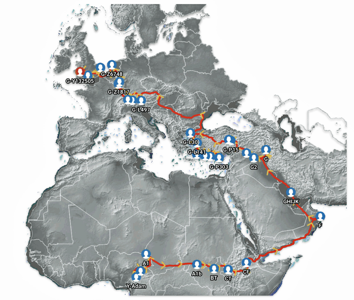
Globetrekker employs sophisticated phylogenetic algorithms that factor in topographical information, historical global sea levels, land elevation, and ice age glaciation. The system combines multiple data types to generate migration paths: archaeological data, earliest known ancestor locations from users and matches, ancient DNA samples, and population genetic studies.
Estes, Roberta, Globetrekker – A New Feature for Big Y Customers from FamilyTreeDNA, 4 Aug 2023, DNAeXplained – Genetic Genealogy, https://dna-explained.com/2023/08/04/globetrekker-a-new-feature-for-big-y-customers-from-familytreedna/
Runfeldt, Goran , Globertrekker, Part 1: A NewFamilyTreeDNA Discover™ Report that Puts Big Y on the Map, 31 Jul 2023, FamilyTreeDNA Blog, https://blog.familytreedna.com/globetrekker-discover-report/
Maier, Paul, Globetrekker, Part 2: Advancing the Science of Phylogeography, 15 Aug 2023, FamilyTreeDNA Blog, https://blog.familytreedna.com/globetrekker-analysis/
[50] Rootsi S, Myres NM, Lin AA, Järve M, King RJ, Kutuev I, Cabrera VM, Khusnutdinova EK, Varendi K, Sahakyan H, Behar DM, Khusainova R, Balanovsky O, Balanovska E, Rudan P, Yepiskoposyan L, Bahmanimehr A, Farjadian S, Kushniarevich A, Herrera RJ, Grugni V, Battaglia V, Nici C, Crobu F, Karachanak S, Hooshiar Kashani B, Houshmand M, Sanati MH, Toncheva D, Lisa A, Semino O, Chiaroni J, Di Cristofaro J, Villems R, Kivisild T, Underhill PA. Distinguishing the co-ancestries of haplogroup G Y-chromosomes in the populations of Europe and the Caucasus. Eur J Hum Genet. 2012 Dec;20(12):1275-82. doi: 10.1038/ejhg.2012.86. Epub 2012 May 16. PMID: 22588667; PMCID: PMC3499744, https://pmc.ncbi.nlm.nih.gov/articles/PMC3499744/
Hay, Maciamo,Haplogroup G2a (Y-DNA), Jul 2023, Eupedia, https://www.eupedia.com/europe/Haplogroup_G2a_Y-DNA.shtml
Haplogroup G-M201, Wikipedia, This page was last edited on 13 January 2025, https://en.wikipedia.org/wiki/Haplogroup_G-M201
Haplogroup G-P303, Wikipedia, This page was last edited on 10 December 2024, https://en.wikipedia.org/wiki/Haplogroup_G-P303
[51] E.K. Khusnutdinova, N.V. Ekomasova, et al., Distribution of Haplogroup G-P15 of the Y-Chromosome Among Representatives of Ancient Cultures and Modern Populations of Northern Eurasia, Opera Med Physiol. 2023. Vol. 10 (4): 57 – 72, doi: 10.24412/2500-2295-2023-4-57-72
Rootsi S, Myres NM, Lin AA, Järve M, King RJ, Kutuev I, Cabrera VM, Khusnutdinova EK, Varendi K, Sahakyan H, Behar DM, Khusainova R, Balanovsky O, Balanovska E, Rudan P, Yepiskoposyan L, Bahmanimehr A, Farjadian S, Kushniarevich A, Herrera RJ, Grugni V, Battaglia V, Nici C, Crobu F, Karachanak S, Hooshiar Kashani B, Houshmand M, Sanati MH, Toncheva D, Lisa A, Semino O, Chiaroni J, Di Cristofaro J, Villems R, Kivisild T, Underhill PA. Distinguishing the co-ancestries of haplogroup G Y-chromosomes in the populations of Europe and the Caucasus. Eur J Hum Genet. 2012 Dec;20(12):1275-82. doi: 10.1038/ejhg.2012.86. Epub 2012 May 16. PMID: 22588667; PMCID: PMC3499744, https://pmc.ncbi.nlm.nih.gov/articles/PMC3499744/
Hay, Maciamo,Haplogroup G2a (Y-DNA), Jul 2023, Eupedia, https://www.eupedia.com/europe/Haplogroup_G2a_Y-DNA.shtml
G-P15 (Y-DNA), Geni, https://www.geni.com/projects/G-P15-Y-DNA/3927
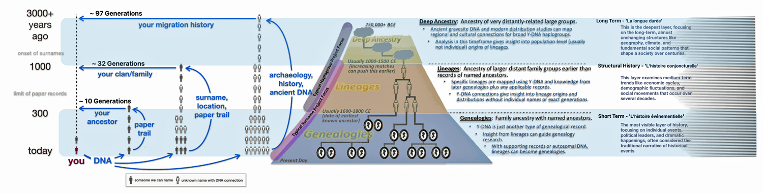
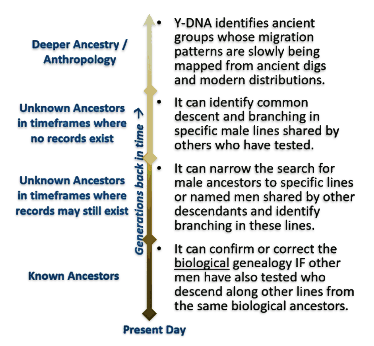
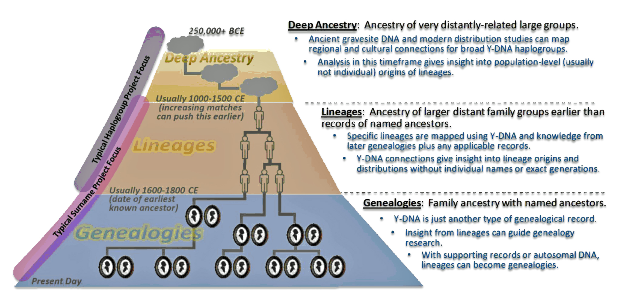
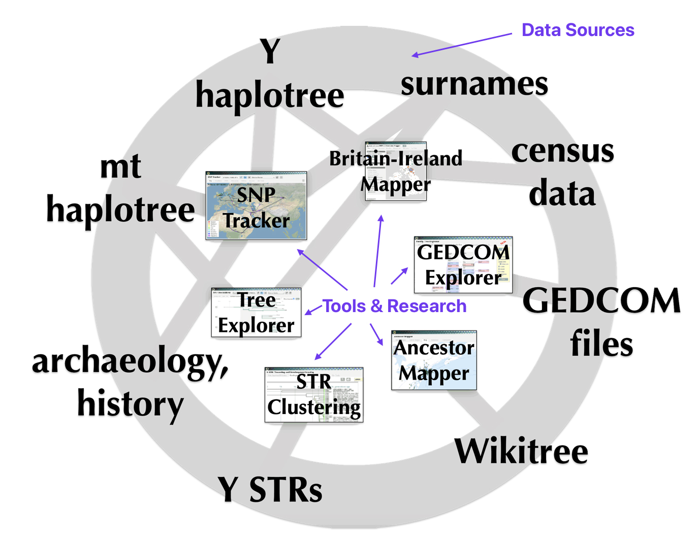
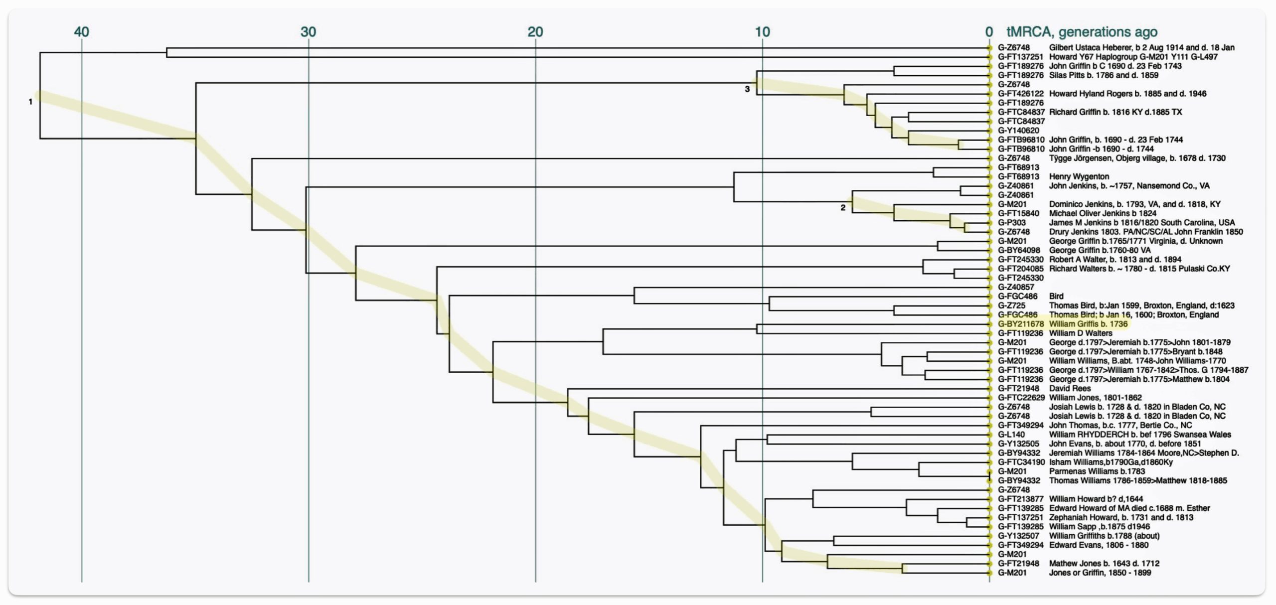

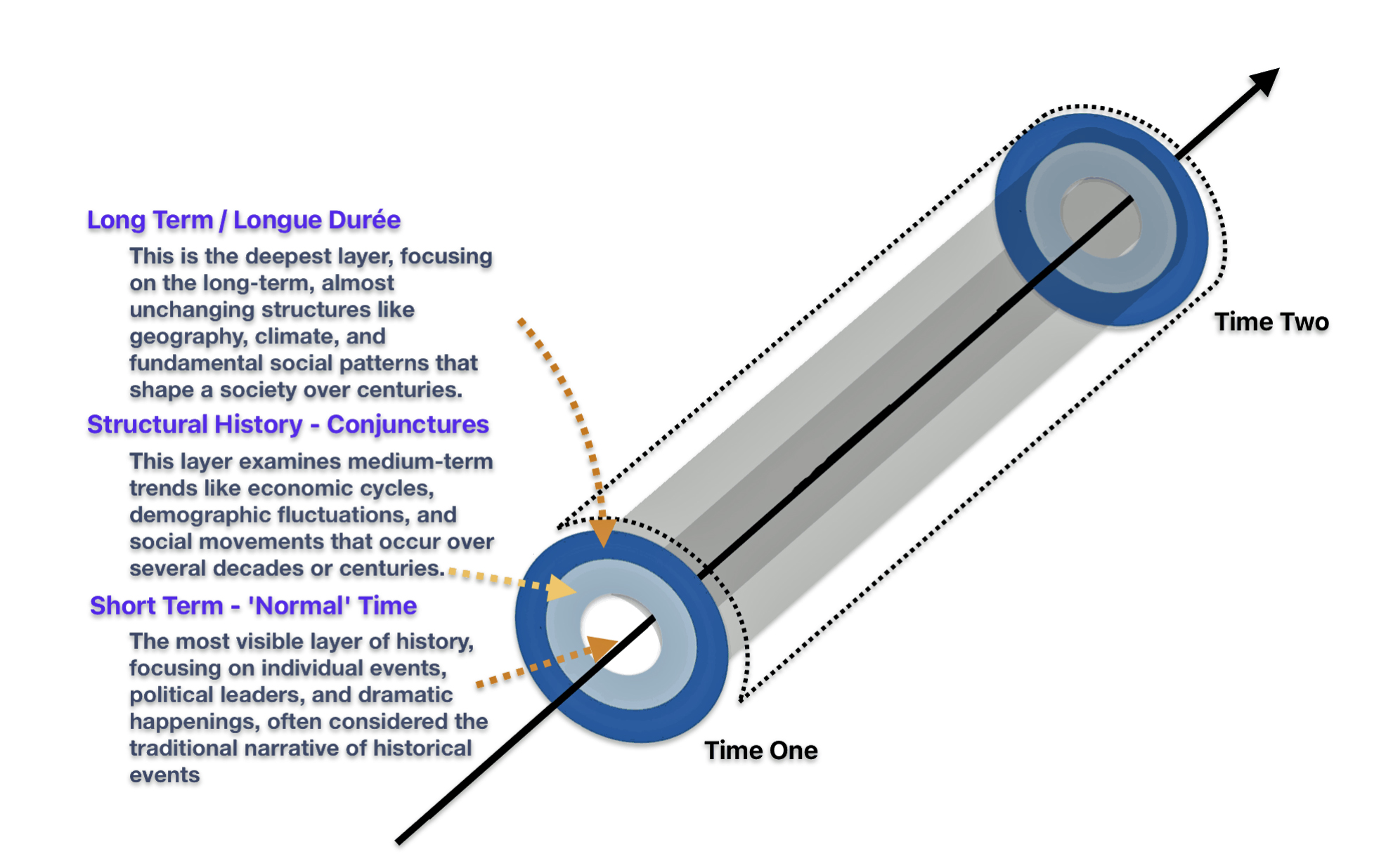

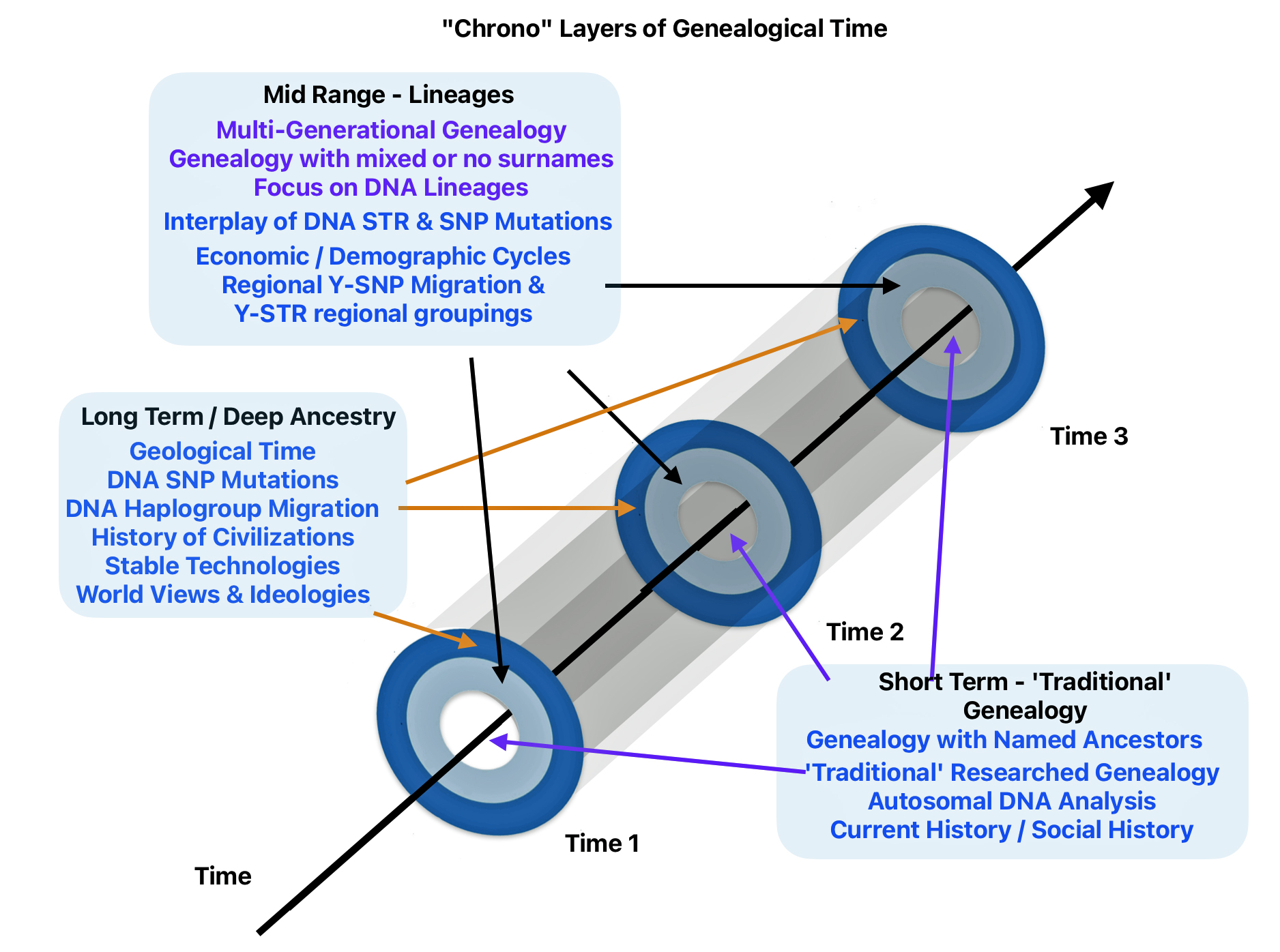
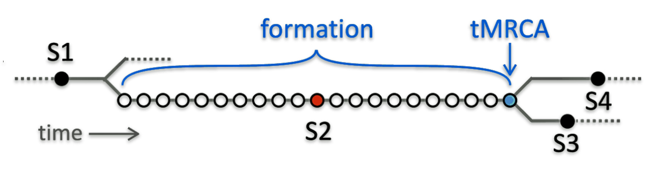
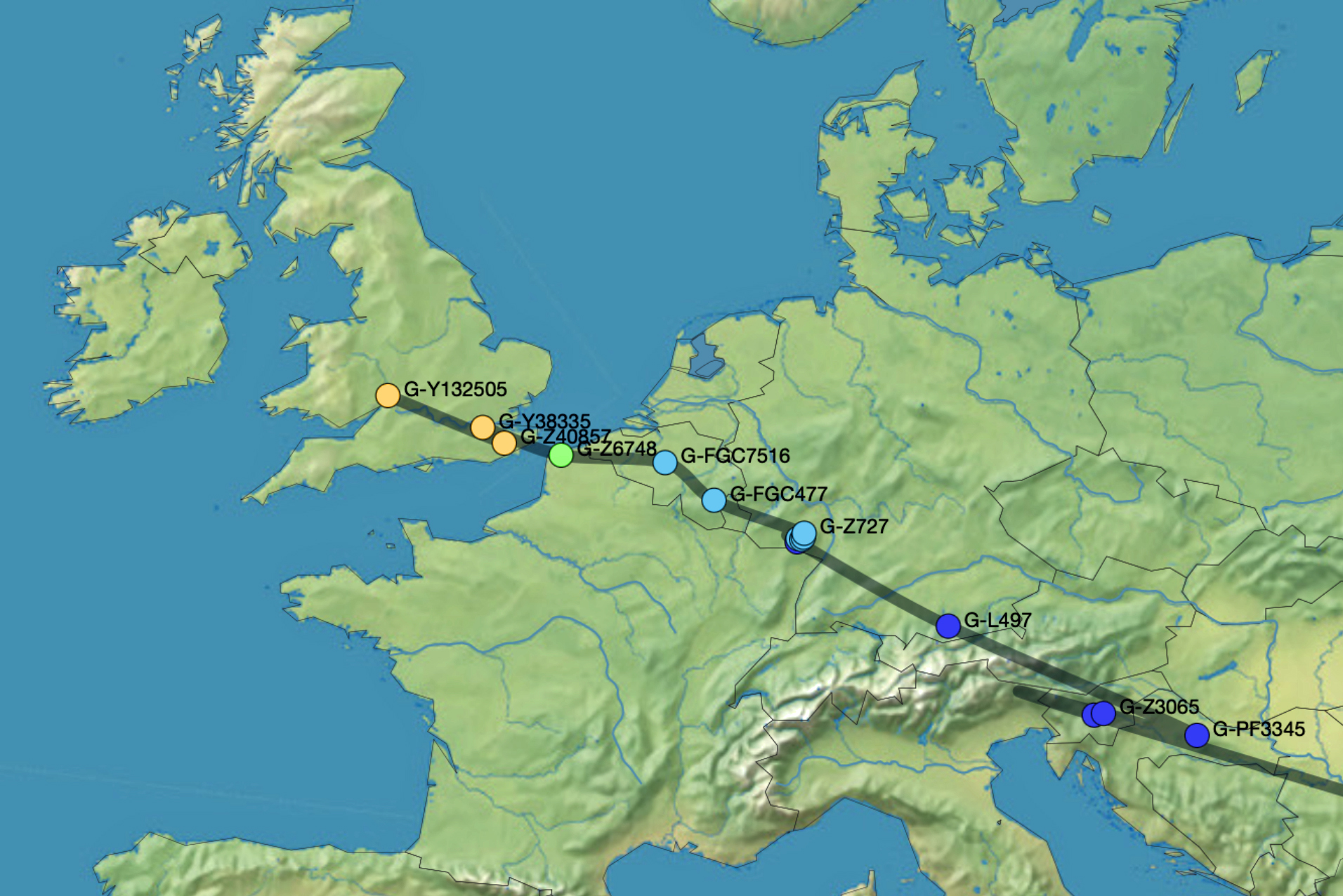