
This story is the second part of a continuation of my focus on the G Haplogroup phylogenetic tree of the Griff(is)(es)(ith) patrilineal line of descent and the migratory route of the Griffis family Y-DNA in the long term genealogical time layer. This second part of the story focuses on two historical periods in the migratory path for the family patrilineal line where the lineage experienced two relatively large time gaps between known haplogroups in the ancestors’ European migratory path. The story discusses common methodological explanations for the absence of haplogroups in each of thee phylogenetic gaps.
These two notable phylogenetic gaps, as indicated in part one of this story, are:
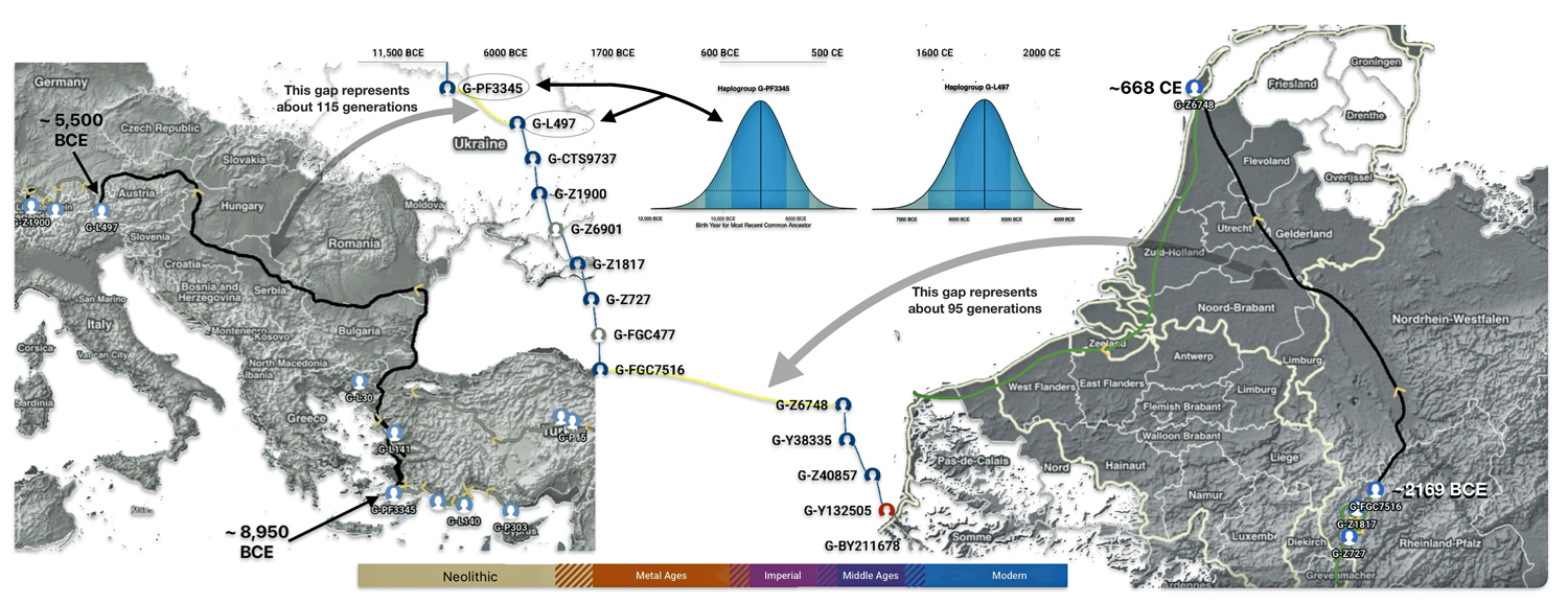
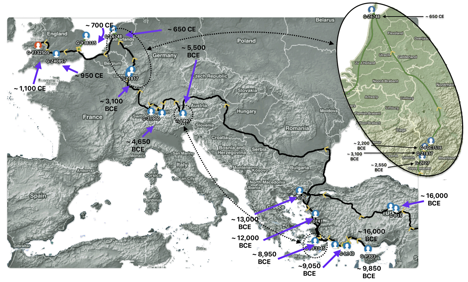
- The 3,450 year Gap between G-PF3345 and G-L497: The common ancestor associated with the haplogroup G-PF3345 was born around 8550 Before Common Era (BCE). He had eleven surviving descendants that were known to have descendants that had unique SNP mutations. The next common ancestor in my YDNA line was associated with the G-L497 haplogroup who was born about 3,500 years later. If we use 30 years as an estimate of a generation, this gap represents about 115 generations. [1]
- The 2,850 year Gap between G-FGC7516 and G-Z6748: This phylogenetic gap was associated with haplogroup G-FGC477. This common ancestor was born around 2200 BCE. He had 6 surviving descendants who had unique SNP mutations. The next genetic ancestor on the Griff(is)(es)(ith) YDNA line was associated with the genetic SNP mutation defining the G-Z6748 haplogroup, 2,850 years later. This gap represents about 95 generations.
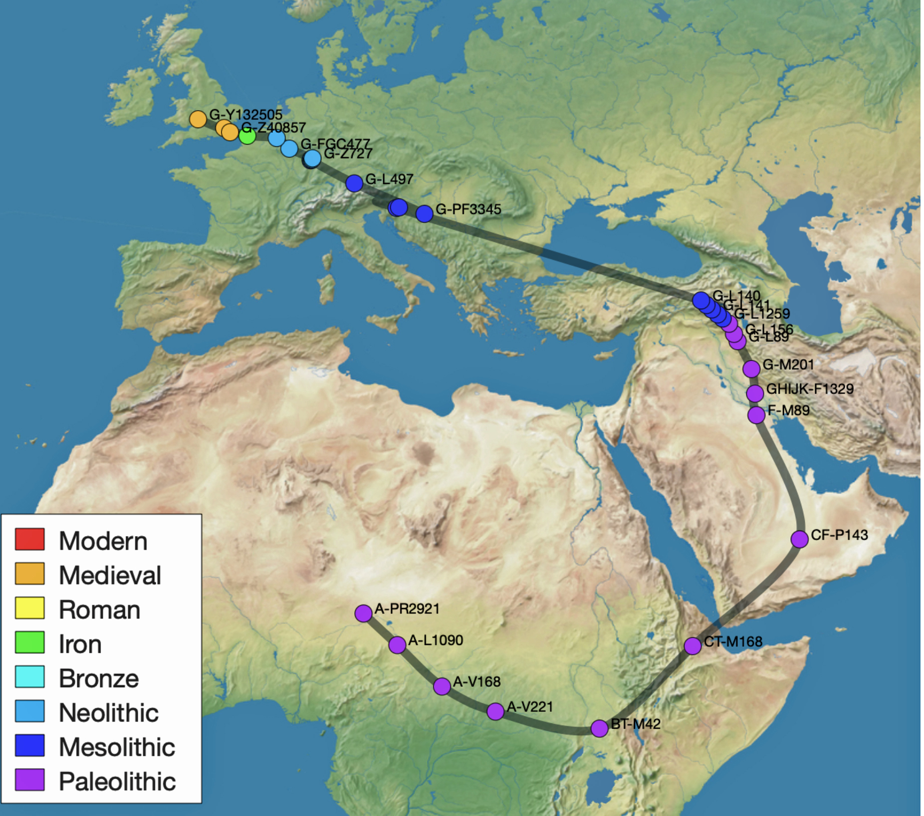
Illustration one provides a graphic portrayal of where each of these phylogenetic gaps reside on the migratory path.
Illustration One: Phylogenetic Time Gaps in the Griff(is)(es)(ith) DNA Migratory Path
General Methodological Explanations for the Phylogenetic Gaps
There are a number of possible explanations for these two phylogenetic gaps that are uniquely tied to demographic, social and historic influences in each of these time periods. However, there also are obvious possible common methodogical explanations for each of the two historical historical gaps in phylogenetic branching. The most straightforward and cogent explanation for these long time gaps is methodologically based.
- Undiscovered Intermediate Subclades
Existing sampling and DNA sequencing efforts may not have captured intermediate haplogroup-defining single nucleotide polymorphisms (SNPs), genetic markers that are used to differentiate haplogroups subclades. Whole-genome sequencing of ancient DNA (aDNA) has revealed that low-coverage studies often miss rare or geographically restricted variants. [2]
For example, the Y chromosome’s repetitive regions and technical challenges in distinguishing true mutations from post-mortem damage in ancient samples can obscure phylogenetic resolution. [3] In addition, the two phylogenetic gaps may harbor uncharacterized branches preserved in understudied populations. [4]
- YDNA Mutation Rate Heterogeneity: Variability in Determining Dates of Haplogroup Subclades
In addition to the absence of subclades in-between these long gaps, mutation rates vary significantly across Y-chromosome haplogroups due to differences in replication timing, chromatin structure, and DNA repair efficiency. [5] Genetic analytical studies have revealed that haplogroups like G exhibit up to 83 percent variability in mutation rates compared to other lineages. [6] This variability in determining birth dates of ancestors associated with haplogroups can create wide gaps between haplogroups.
A slowdown in the mutation rate along these two areas of the G phylogenetic tree where there is a significant gap could artificially extend MRCA or haplogroup estimates. This hypothesis aligns with studies showing that high-coverage sequencing detects 10–17 times more mutations than low-coverage methods, suggesting earlier TMRCA (the most recent common ancestor) calculations may overestimate divergence times. [7]
The magnitude of time associated with the two phylogenetic gaps are influenced by the estimated date of the endpoints of each gap – namely the estimate birth date of the haplogroup subclades. The dating of Y-DNA haplogroups, estimating when specific branches of the paternal lineage tree arose, is based on genetic mutations that accumulate over generations.
Y-DNA haplogroups are defined by unique single-nucleotide polymorphism (SNP) mutations. Each SNP acts as a “time-and-date stamp” on the Y chromosome, marking a branch point in the paternal lineage tree. By counting the number of SNP mutations from a known ancestor and applying an estimated mutation rate (how often such mutations occur per generation or per year), researchers estimate the coalescence age.
In genetics, coalescence age refers to the estimated time to the most recent common ancestor (TMRCA) of a set of genetic lineages. It represents the number of generations that have passed since those lineages shared a common ancestor. This concept is central to the coalescent theory, which models the genealogical relationships between genes in a population. [8]
The coalescence age is determined by statistical models that estimate when the most recent common ancestor (tMRCA) of all men in a haplogroup lived, based on the observed genetic diversity and mutation rates. Improved models and larger datasets have refined these age estimates over time.
Confidence intervals (CIs) for Y-DNA haplogroup dates quantify the uncertainty in estimating when a specific paternal lineage arose. These intervals are calculated using statistical models that incorporate mutation rates, genetic diversity, and sample size. Typically three confidence intervals are provided for the age of haplogroups: [9]
Table One: Confidence Invervals for Most Recent Common Ancestor Births
| Confidence Interval (CI) | Description |
|---|---|
| 68 Percent | Narrow range with a 32 percent chance the true age lies outside it (higher precision, lower confidence) |
| 95 Percent | Wider range, capturing 95 percent of probable ages (commonly used in genealogical studies) |
| 99 Percent | Broadest range, accounting for extreme outliers |
Tools like FamilyTreeDNA’s FTDNATiPTM report automate these calculations, providing genealogists with probabilistic age ranges for ancestral connections. [10]
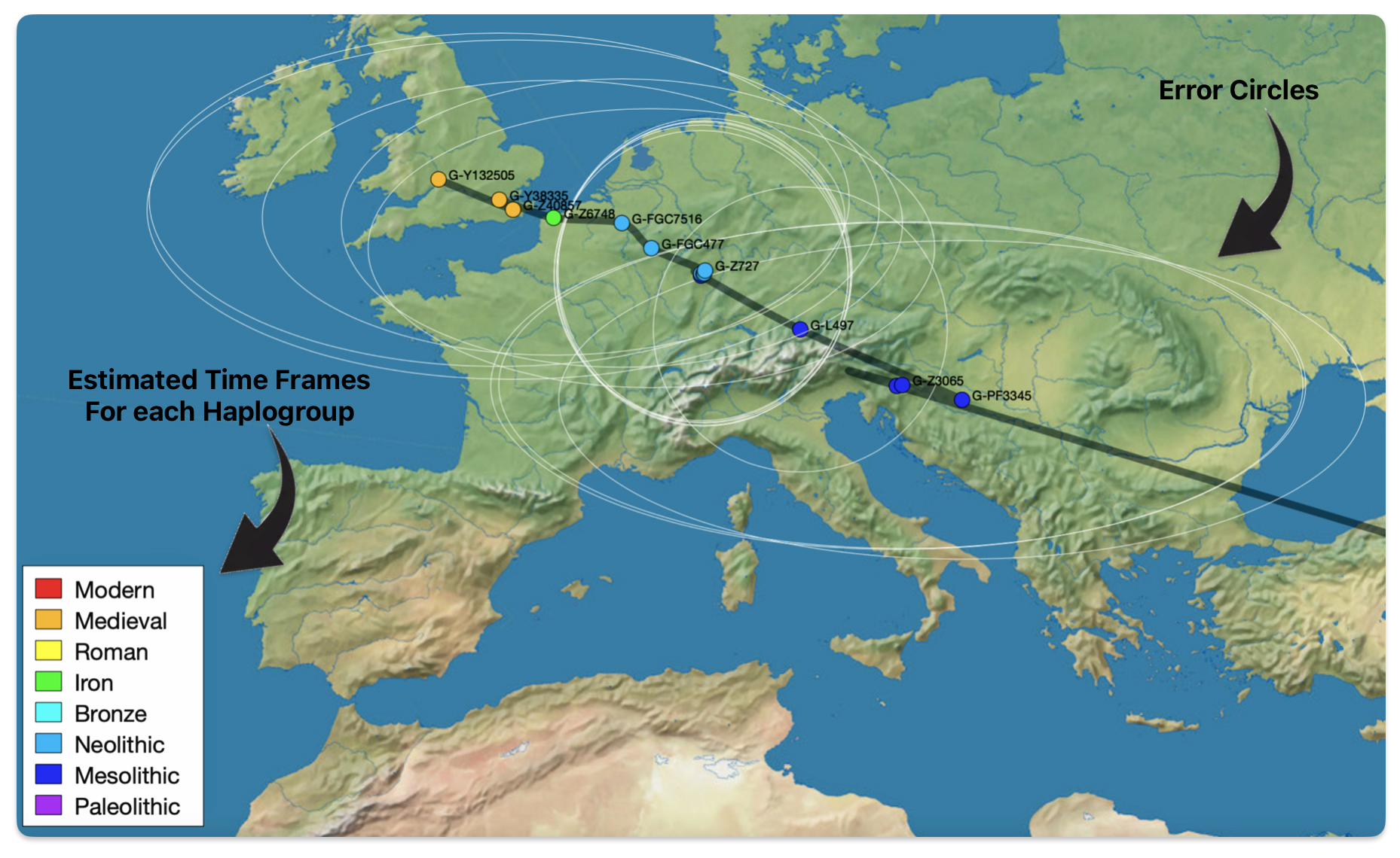
Illustration two provides an example of one of the endpoints of the first phylogenetic gap. It is estimated that the individual associated with this haplgroup was born around 8971 BCE. Statistically, we are 99 percent confident that he was born between 11,375 BCE and 6874 BCE. This represents four thousand and five hundred years which is a large swath of time to ‘pinpoint’ his estimated birth. This 99 percent confidence inteval is larger than the time gap we are examining!
Illustration Two: Example of Estimated Birth Year for the Most Recent Common Ancestor Associated with G-PF3345
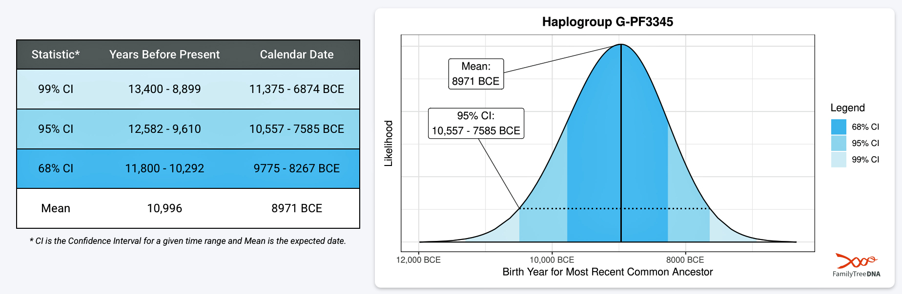
If we were to utilize the 95 percent CI estimate, this would place the ancestor’s birth between 10,557 BCE and 7,585 BCE.
Depending on what birth date value one uses, the phylogenetic gap could be very narrow or very expansive. Using a tighter confidence interval is usually more useful despite the increase in potential error in reliability. I have utilized the mean value and the 68 percent confidence interval for estimated birth dates for ancestors associated with specific haplogroups.
- Temporal Discontinuities in Ancient DNA Sampling
The archaeological record of haplogroup G is sparse relative to other major haplogroups. Most ancient G2a specimens derive from Early Neolithic sites, while later samples are underrepresented. This sampling bias creates a false impression of stasis. Recent aDNA studies highlight the need for broader geographic and temporal coverage to resolve such gaps. [11]
- Long Branch Phylogenetics
When a Y-DNA phylogenetic tree displays few subclades over a long stretch of time, geneticists call this a “long branch” – a significant period where little apparent diversification occurred in the paternal lineage. This pattern suggests a lineage survived through challenging conditions before eventually flourishing. The G haplogroup demonstrates this characteristic in numberous situations, with some branches having notably long branches and deep-rooting nodes. [12]
An evolutionary bottleneck, also known as a genetic or population bottleneck, is a sharp reduction in the size of a population that leads to significant loss of genetic diversity. This phenomenon occurs when a population is dramatically reduced due to environmental catastrophes, habitat destruction, disease outbreaks, or human activities. [13]
- Challenges in predicting geographic location from genetic variation
In a number of my stories, I have utilized two innovative tools designed to visualize the migration paths of haplogroups based on genetic data: SNP Tracker and GlobetrekkerTM. Illustration one above is an example of a using the FamilyTreeDNA Globetrekker mapping tool. Each of the graphing software use samples of Single Nucleotide Polymorphisms (SNPs) from Y-DNA and mitochondrial DNA (mtDNA) to trace ancestral routes from ancient times to the present. (Graphically depicted in illustration three.) Both of these tools integrate data from FamilyTreeDNA’s YDNA and mtDNA databases. They also utilize ancient DNA (aDNA) samples, allowing users to explore the historical journey of their genetic lineage through time and space.
Illustration Three: Depiction of Geographic Location and Genetic Variation
The accuracy of SNP tracking programs, such as the SNP Tracker and GlobeTrekkerTM [14], in predicting migration patterns varies depending on the methodology, data quality, and the complexity of genetic and geographic factors. (See illustration four.) While these tools provide valuable insights, they have limitations that affect their precision. Both tools highlight geographical variance but caution against overinterpreting precise locations. For deeper analysis, combining both tools with archaeological and historical records yields the most robust insights.
Illustration Four: Comparison of SNP Tracker and Globetrekker Maps for Griff(is)(es)(ith YDNA Migration
SNP tracking programs are reasonably accurate for predicting general migration patterns when sufficient training data and dense SNP arrays are available. However, their accuracy diminishes with sparse datasets, biased sampling, or complex genetic structures. Researchers must account for these limitations by combining SNP tracking tools with complementary methods (e.g., archaeological evidence or environmental modeling) to achieve more robust migration reconstructions. [15]
SNP tracking programs like Rob Spencer’s SNP Tracker and FTDNA’s Globetrekker incorporate geographical variance and uncertainty when modeling migration patterns. It should be noted that their approaches differ.
The SNP Tracker uses various data types to infer SNP locations: ancient DNA sources such as the Allen Ancient DNA Resource (AADR), Carlos Quiles’ Ancient DNA Database, Maciamo Hay’s Eupedia, and Wikipedia sources. It uses Tom Patterson’s mapping at Natural Earth and Shaded Relief. [16] The SNP Tracker relies on FamilyTreeDNA’s extended DNA and mtDNA Database. Spencer’s SNP migration maps acknowledge uncertainty through “error circles” on maps, reflecting limited data resolution. Spencer emphasizes that results are averages of scattered data and subject to revision as new evidence emerges. [17]
Illustration five depicts a ‘zoom in’ view of Europe in the SNP Tracker with the white circles of confidence. In fairness to the quality of the SNP tracker program, enabling the zoom in function on Europe distorts the earlier migratory path from Asia Minor.
Illustration five: SNP Tracker Results for Griff(is)(es)(ith) Migration Route
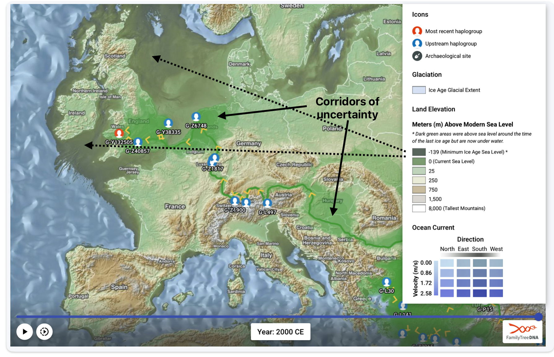
The FTDNA GlobeTrekker program integrates environmental factors (e.g., elevation, glaciation, sea levels) and anthropological data to model “most likely” migration corridors. The generated maps also depict areas of land (e.g. Doggerland) that subsequently were submerged after the glacial period. It anchors around 100 haplogroups using ancient DNA and archaeological coordinates, reducing reliance on modern tester bias. Globetrekker also relies on FamilyTreeDNA’s extended DNA and mtDNA Database. The uncertainy of migration routes are shown with shaded ‘corridors’ of uncertainty‘. (See illustration six.)
Illustration Six: Globetrekker Results for Griff(is)(es)(ith) Migration Route
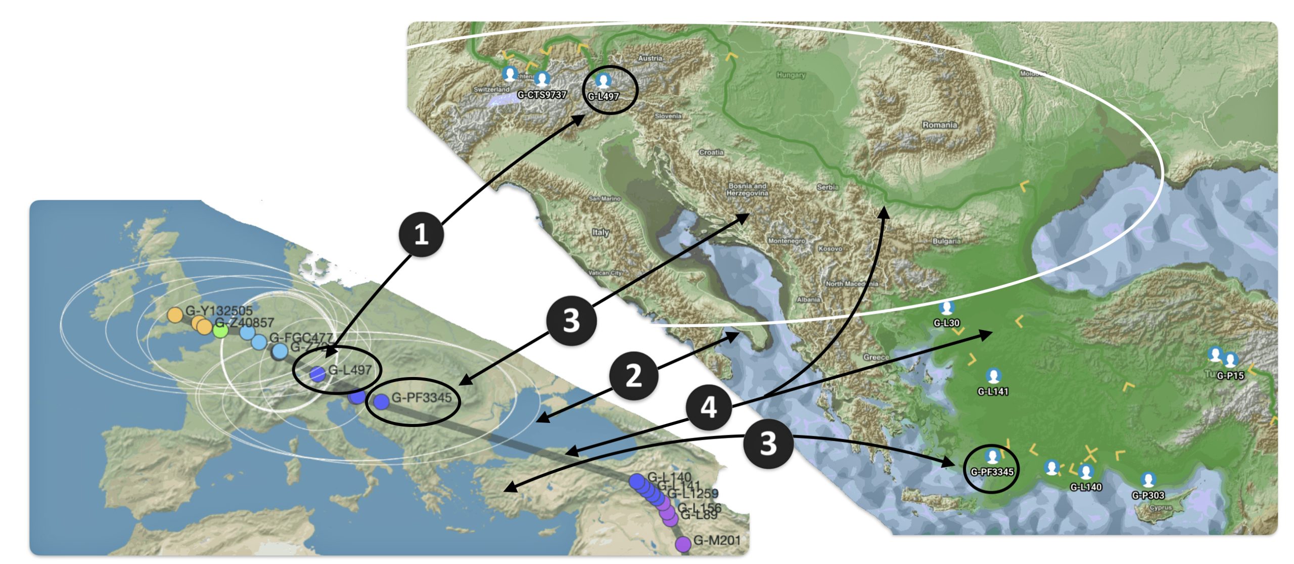
Both tools highlight geographical variance but caution against overinterpreting precise locations. Users are advised to treat results as approximations with error margins, especially for older haplogroups. An example of how the respective migration models produce different geographical conclusions is to compare the estimated locations and estimated migratory paths of the two phylogenetic gaps between haplogroups G-PF3345 and G-L497; and between haplogroups G-FGC7516 and G-Z6748.
Illustration seven depicts the differences in geographical location of haplogroups G-PF3345 and G-L497 between the two mapping programs. The SNP tracker map is in the lower left hand corner of the illustration and the Globetrekker map is located in the upper right hand corner of the illustration. In general, notwithstanding the geographical variance in each of the programs’ calcuations, the Globetrekker mapping program appears to provide a more defined migratory path between the two haplogroups, especially for older haplogroups.
Illustration Seven: Comparison of SNP Tracker and Globetrekkers’ Depiction of Locations of G-PF3345 and G-L497
The following observations, as numbered one through four in illustration seven above, are provided:
- The geographical location of haplogrup G-L497 is relatively consistent between the two mapping programs.
- SNP Tracker’s circle of error for the location of haplogroup G-PF3345 is very large and coveres most of sourthern Europe. The white circle is also depicted on the Globetrekker map.
- The approximate geographical location of haplogroup G-PF3345 is substantially different between the two mapping programs. For the SNP Tracker, the haplogroup’s estimated location is where modern day Croatia is situated. Globetrekker estimated its location in modern day Turkey or ancient Anatolia.
- The estimated migratory path is broadly defined in the SNP Tracker map. The migratory path in the Globetrekker path is more detialed, even within the shaded ‘corridors’ of uncertainty.
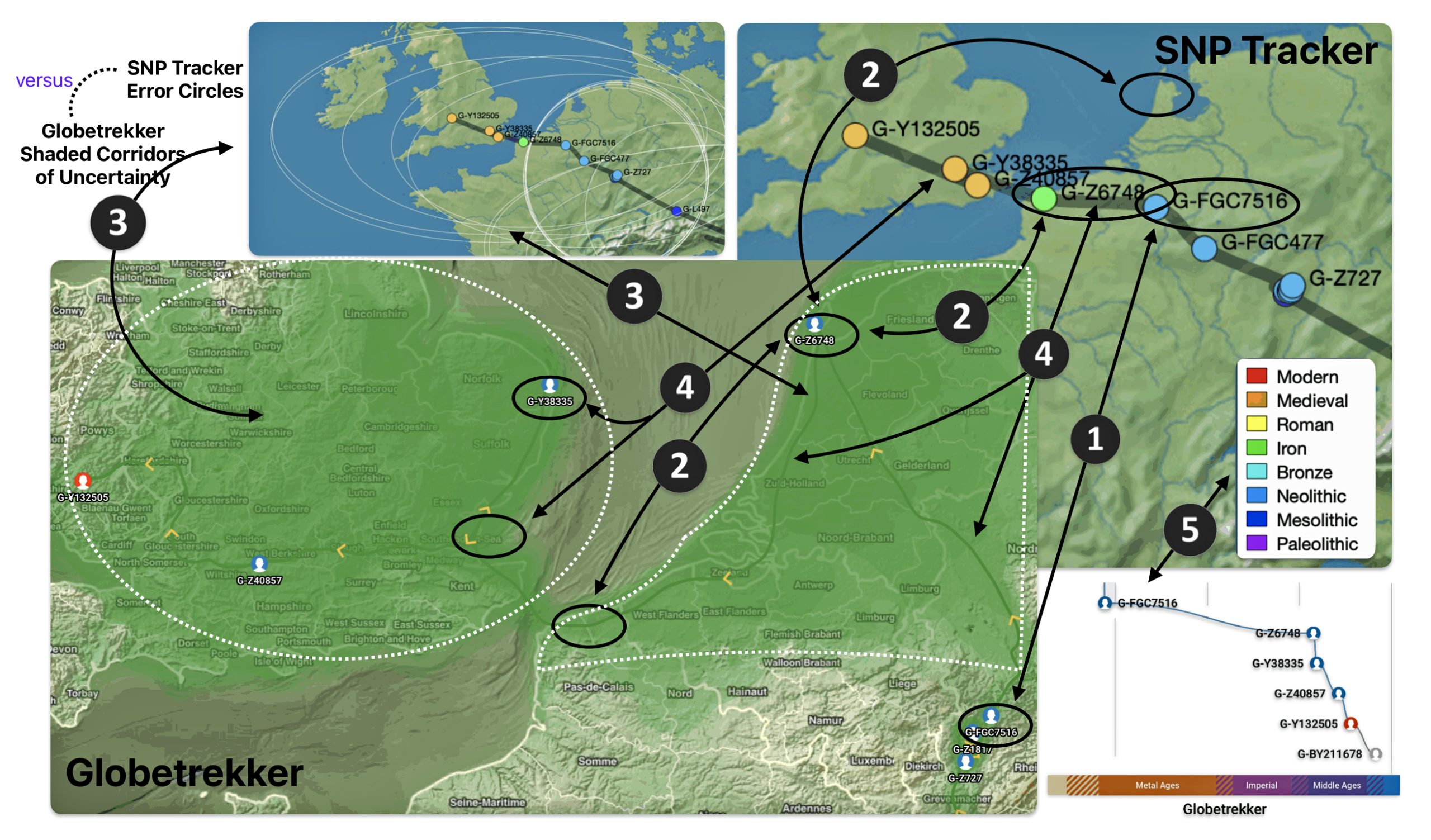
Illustration eight depicts the differences in geographical location of haplogroups G-FGC7516 and G-Z6748. The SNP tracker map is in the upper right hand corner of the illustration and the Globetrekker map is located in the lower left hand corner of the illustration. In general, the Globetrekker mapping program appears to provide a more defined migratory path between the two haplogroups.
Illustration Eight: Comparison of SNP Tracker and Globetrekkers’ Depiction of Locations of G-FGC7516 and G-Z6748
The following observations, as numbered one through five in illustration eight, are provided:
- The geographical location of haplogrup G-FGC7516 is relatively consistent between the two mapping programs.
- The estmated gengraphical location of haplogroup G-Z6748 resulted in different locations in each of the mapping programs. For the SNP Tracker program, the ancestor associated with the G-Z6748 haplogroup resided further down the European coast than what is depicted in the Globetrekker map.
- The range of predictive eror associated with predicting the geographical location of haplogroup G-Z6748 is broader in the SNP Tracker map than the Globetrekker map. While the shaded corridors of uncertainty in the in the Globetrekker map are more specific, they still account for the possibility of G-Z6748 located where the SNP Tracker identified its location.
- The estimated migratory path is broadly defined in the SNP Tracker map. The migratory path in the Globetrekker path is more detialed, even within the shaded ‘corridors’ of uncertainty.
- Each mapping program estimates different time periods associated with each haplgroup. when the genetic line cross the channel to the British Isle. SNP Tracker esitmates that the YDNA line crossed over in Roman times. The GlobeTrekker program estimates the crossing occured in the medieval time.
Rob Spencer’s SNP Tracker and FamilyTreeDNA’s Globetrekker both use historical time categories to situate haplogroups, but their periodization and terminology differ slightly. Table two provides a comparison of the time categories used by each tool and their approximate date ranges.
Table Two: Comparison of Time Peiods Used in the SNP Tracker and the Globetreker Mapping Programs
| SNP Tracker Category | Approximate Dates (Europe/West Asia) | Globetrekker Category | Approximate Dates (Europe/West Asia) |
|---|---|---|---|
| Neolithic | 10,000–3,300 BCE | Metal Ages | 6,000–1,000 BCE (Copper, Bronze, Iron Ages) |
| Bronze | 3,300–1,200 BCE | Metal Ages | 6,000–1,000 BCE |
| Iron | 1,200–500 BCE | Metal Ages | 6,000–1,000 BCE |
| Roman | 27 BCE–476 CE | Imperial | 27 BCE–284/375 CE |
| Medieval | 500–1500 CE | Medieval | 500–1500 CE |
| Modern | 1500 CE–present | (Not explicitly named; post-medieval implied) | 1500 CE–present (implied) |
The following are key points of comparison:
- Neolithic (SNP Tracker): Refers to the New Stone Age, preceding the widespread use of metals. Globetrekker does not use this term explicitly, instead grouping later prehistory under ‘Metal Ages’.
- Bronze and Iron (SNP Tracker): SNP Tracker splits the Metal Ages into Bronze and Iron, while Globetrekker combines them under ‘Metal Ages’.
- Roman/Imperial: Both tools have a category for the Roman/Imperial period, generally spanning the Roman Empire’s dominance in Europe.
- Medieval: Both use ‘Medieval’ for the Middle Ages, with similar date ranges.
- Modern: SNP Tracker includes a ‘Modern’ category for the post-medieval era, while Globetrekker’s categories typically end at ‘Medieval’, with modern times implied but not explicitly labeled.
Part Three of the Story
The story continues with a discussion of the possible social and cultural explanations of the two phylogenetic gaps in the migratory history of the Griff(is)(es)(ith) patrilinal line.
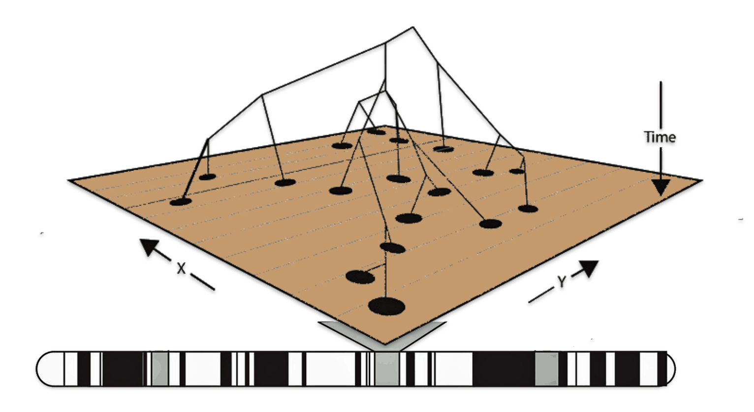
Feature Banner: The banner at the top of the story is a modification of a shapshot taken from the FamilyTreeDNA GlobetrekkerTM video of the migratory path of my YDNA descendants over time. The map shows the maigratory path of selected most common recent ancestors and their respective eestimated dates of birth. In addition the map highlights two time periods where there was a signficant time period in between haplogroups that are discussed in the present story.
[1] In ancient DNA analysis, a generation is typically associated with a span of 26 to 30 years. This estimate is derived from genetic methods that compare recombination events and mutation rates in ancient genomes to those of contemporary humans. Multiple studies using both recombination and mutation clocks have consistently found that the mean human generation interval over the past 45,000 years falls within this 26–30 year range.
This interval is considered a “sex-averaged” value, reflecting both male and female reproductive ages averaged across populations and time periods. While the generation time has varied slightly due to historical and environmental factors, the 26–30 year estimate is robust and widely used for dating ancient samples and calibrating molecular clocks in human evolutionary studies.
Richard J. Wang et al. ,Human generation times across the past 250,000 years.Sci. Adv.9,eabm7047(2023).DOI:10.1126/sciadv.abm7047
Priya. Moorjani, Sriram Sankararaman, Qiaomei Fu, Molly Przeworski, Nick Patterson, and David Reich, A genetic method for dating ancient genomes provides a direct estimate of human generation interval in the last 45,000 years, Proc. Natl. Acad. Sci. U.S.A. 113 (20) 5652-5657,https://doi.org/10.1073/pnas.1514696113 (2016).
[2] Kivisild T. The study of human Y chromosome variation through ancient DNA. Hum Genet. 2017 May;136(5):529-546. doi: 10.1007/s00439-017-1773-z. Epub 2017 Mar 4. Erratum in: Hum Genet. 2018 Oct;137(10):863. doi: 10.1007/s00439-018-1937-5. PMID: 28260210; PMCID: PMC5418327, (PubMed) https://pmc.ncbi.nlm.nih.gov/articles/PMC5418327/
[3] Ibid
[4] The enigma of G-PF3345 (U1, CTS342 and L497), 3 Sep 2018, G2a, YDNA Haplogroups, Population Genetics, Forums, Eupedia, https://www.eupedia.com/forum/threads/the-enigma-of-g-pf3345-u1-cts342-and-l497.37040/
Boed Marres, , 19 Feb 2025, G-M201, Marres, https://www.marres.nl/EN/G-M201.htm
[5] Ding Q, Hu Y, Koren A, Clark AG. Mutation Rate Variability across Human Y-Chromosome Haplogroups. Mol Biol Evol. 2021 Mar 9;38(3):1000-1005. doi: 10.1093/molbev/msaa268. PMID: 33049047; PMCID: PMC7947773, (PubMed) https://pmc.ncbi.nlm.nih.gov/articles/PMC7947773/
Jeanson, Nathaniel, Evidence for a Human Y Chromosome Molecular Clock: Pedigree-Based Mutation Rates Suggest a 4,500-Year History for Human Paternal Inheritance, Answers Research Journal 12 (2019) 393–404. www.answersingenesis.org/arj/v12/human_y_chromosome_molecular_clock.pdf
[6] Ding Q, Hu Y, Koren A, Clark AG. Mutation Rate Variability across Human Y-Chromosome Haplogroups. Mol Biol Evol. 2021 Mar 9;38(3):1000-1005. doi: 10.1093/molbev/msaa268. PMID: 33049047; PMCID: PMC7947773, (PubMed) https://pmc.ncbi.nlm.nih.gov/articles/PMC7947773/
[7] Jeanson, Nathaniel, Evidence for a Human Y Chromosome Molecular Clock: Pedigree-Based Mutation Rates Suggest a 4,500-Year History for Human Paternal Inheritance, Answers Research Journal 12 (2019) 393–404. www.answersingenesis.org/arj/v12/human_y_chromosome_molecular_clock.pdf ; see also https://answersresearchjournal.org/evidence-y-chromosome-molecular-clock/
[8] Coalescent Theory, Wikipedia, This page was last edited on 15 December 2024, https://en.wikipedia.org/wiki/Coalescent_theory
[9] Key Factors in caluculating confdence intervals are:
Mutation Rate Uncertainty: The Y chromosome’s mutation rate (for SNPs or STRs) is estimated through pedigree studies, ancient DNA, or evolutionary comparisons (e.g., human-chimpanzee divergence). These rates often have their own confidence intervals.
Calibration with External Data: Archaeological or historical events (e.g., Sardinian population expansion ~7.7 kya) anchor haplogroup dates, narrowing confidence intervals when available.
Sample Size and Data Distribution: Sample size and data distribution have an impact on estimating haplogrup dates. Larger datasets reduce uncertainty. For small groups, Poisson noise dominates; for large groups, mutation rate accuracy becomes critical. [7c] FamilyTreeDNA’s FTDNATiPTM report uses thousands of Y-STR matches to generate CIs. A genetic distance of 2 at 37 markers might produce a 95% confidence interval of 500–1,300 years.
Genetic Diversity Analysis: The number of mutations observed in a haplogroup’s lineage is compared to the mutation rate. Statistical models (e.g., coalescent theory) estimate the time to the most recent common ancestor (TMRCA).
See: Wang CC, Gilbert MT, Jin L, Li H. Evaluating the Y chromosomal timescale in human demographic and lineage dating. Investig Genet. 2014 Sep 10;5:12. doi: 10.1186/2041-2223-5-12. PMID: 25215184; PMCID: PMC4160915, (PubMed) https://pmc.ncbi.nlm.nih.gov/articles/PMC4160915/
García-Fernández, C., Lizano, E., Telford, M. et al. Y-chromosome target enrichment reveals rapid expansion of haplogroup R1b-DF27 in Iberia during the Bronze Age transition.Sci Rep 12, 20708 (2022). https://doi.org/10.1038/s41598-022-25200-7
Wang CC, Gilbert MT, Jin L, Li H. Evaluating the Y chromosomal timescale in human demographic and lineage dating. Investig Genet. 2014 Sep 10;5:12. doi: 10.1186/2041-2223-5-12. PMID: 25215184; PMCID: PMC4160915, PubMed) https://pmc.ncbi.nlm.nih.gov/articles/PMC4160915/
McDonald I. Improved Models of Coalescence Ages of Y-DNA Haplogroups. Genes (Basel). 2021 Jun 4;12(6):862. doi: 10.3390/genes12060862. PMID: 34200049; PMCID: PMC8228294, (PubMed) https://pmc.ncbi.nlm.nih.gov/articles/PMC8228294/
[10] Y-DNA FTDNATiP™ Report Introduction, FamilyDNADNA Help center, https://help.familytreedna.com/hc/en-us/articles/6162096082831-Y-DNA-FTDNATiP-Report-Introduction
Estes, Roberta, FamilyTreeDNA DISCOVER™ Launches – Including Y DNA Haplogroup Ages, 30 Jun 2022, DNAeXplained – Genetic Genealogy, familytreedna-discover-launches-including-y-dna-haplogroup-ages
[11] Kivisild T. The study of human Y chromosome variation through ancient DNA. Hum Genet. 2017 May;136(5):529-546. doi: 10.1007/s00439-017-1773-z. Epub 2017 Mar 4. Erratum in: Hum Genet. 2018 Oct;137(10):863. doi: 10.1007/s00439-018-1937-5. PMID: 28260210; PMCID: PMC5418327, (PubMed) https://pmc.ncbi.nlm.nih.gov/articles/PMC5418327/
[12] Qu, XJ., Jin, JJ., Chaw, SM. et al. Multiple measures could alleviate long-branch attraction in phylogenomic reconstruction of Cupressoideae (Cupressaceae). Sci Rep 7, 41005 (2017). https://doi.org/10.1038/srep41005
Roch S, Nute M, Warnow T. Long-Branch Attraction in Species Tree Estimation: Inconsistency of Partitioned Likelihood and Topology-Based Summary Methods. Syst Biol. 2019 Mar 1;68(2):281-297. doi: 10.1093/sysbio/syy061. PMID: 30247732, PubMed) https://pubmed.ncbi.nlm.nih.gov/30247732/
Swiel, Y., Kelso, J. & Peyrégne, S. Resolving the source of branch length variation in the Y chromosome phylogeny. Genome Biol 26, 4 (2025). https://doi.org/10.1186/s13059-024-03468-4
[13] Population bottleneck, Wikipedia, This page was last edited on 25 March 2025, https://en.wikipedia.org/wiki/Population_bottleneck
[14] Spencer, Rob, SNP Tracker, Scaled Inovation, https://scaledinnovation.com/gg/snpTracker.html
Estes, Roberta, Globetrekker – A New Feature for Big Y Customers from FamilyTreeDNA, 4 Aug 2023, DNAeXplained – Genetic Genealogy, https://dna-explained.com/2023/08/04/globetrekker-a-new-feature-for-big-y-customers-from-familytreedna/
Runfeldt, Goran , Globertrekker, Part 1: A NewFamilyTreeDNA Discover™ Report that Puts Big Y on the Map, 31 Jul 2023, FamilyTreeDNA Blog, https://blog.familytreedna.com/globetrekker-discover-report/
Maier, Paul, Globetrekker, Part 2: Advancing the Science of Phylogeography, 15 Aug 2023, FamilyTreeDNA Blog, https://blog.familytreedna.com/globetrekker-analysis/
Vilar, Miguel, Globetrekker, Part 3: We Are Making History, 26 Sep 2023, FamilyTreeDNA Blog, https://blog.familytreedna.com/globetrekker-history/
[15] CJ Battey, Peter L Ralph, Andrew D Kern, Predicting geographic location from genetic variation with deep neural networks eLife 9:e54507. 2020, https://doi.org/10.7554/eLife.54507
Leaché D. , Adam and Jamie R. Oaks, The Utility of Single Nucleotide Polymorphism (SNP) Data in Phylogenetics, Annual Review of Eccology, Evolution and Systematics, 20176, 48:69-84, https://www.annualreviews.org/content/journals/10.1146/annurev-ecolsys-110316-022645
[16] The following are a few of the sources Spencer utilized to develop the SNP Tracker:
Mallick, S., Micco, A., Mah, M. et al. The Allen Ancient DNA Resource (AADR) a curated compendium of ancient human genomes. Sci Data 11, 182 (2024). https://doi.org/10.1038/s41597-024-03031-7
Mallick S, Micco A, Mah M, Ringbauer H, Lazaridis I, Olalde I, Patterson N, Reich D. The Allen Ancient DNA Resource (AADR): A curated compendium of ancient human genomes. bioRxiv [Preprint]. 2023 Apr 6:2023.04.06.535797. doi: 10.1101/2023.04.06.535797. Update in: Sci Data. 2024 Feb 10;11(1):182. doi: 10.1038/s41597-024-03031-7. PMID: 37066305; PMCID: PMC10104067, (PubMed) https://pubmed.ncbi.nlm.nih.gov/37066305/
Quiles, Carlos and Jean Manco, Ancient Y-DNA and mtDNA, 2020, https://indo-european.eu/ancient-dna/
Quiles, Carlos and Jean Manco, Prehistory Atlas, https://indo-european.eu/maps/
Tom Sommers, Great Rivers of Europe, Euro Canals, https://eurocanals.com/Rivers/great-rivers-of-europe.html
[17] See Sources Tab on the SNP Tracker Results Page, Rober Spencer, SNP Tracker, Scaled Inovation, https://scaledinnovation.com/gg/snpTracker.html